Benchmarking pipeline

Biological activities can be estimated by coupling a statistical method with a prior knowledge network. However, it is not clear which method or network performs better. When perturbation experiments are available, one can benchmark these methods by evaluating how good are they at recovering perturbed regulators. In our original decoupler publication, we observed that wsum, mlm, ulm and consensus where the top performer methods.

In this notebook we showcase how to use decoupler for the benchmarking of methods and prior knowledge networks. The data used here consist of single-gene perturbation experiments from the KnockTF2 database, an extensive dataset of literature curated perturbation experiments. If you use these data for your resarch, please cite the original publication of the resource:

Chenchen Feng, Chao Song, Yuejuan Liu, Fengcui Qian, Yu Gao, Ziyu Ning, Qiuyu Wang, Yong Jiang, Yanyu Li, Meng Li, Jiaxin Chen, Jian Zhang, Chunquan Li, KnockTF: a comprehensive human gene expression profile database with knockdown/knockout of transcription factors, Nucleic Acids Research, Volume 48, Issue D1, 08 January 2020, Pages D93–D100, https://doi.org/10.1093/nar/gkz881

Note

This tutorial assumes that you already know the basics of decoupler. Else, check out the Usage tutorial first.

Loading packages

First, we need to load the relevant packages.

import pandas as pd
import numpy as np
import matplotlib.pyplot as plt

import decoupler as dc

Loading the data

We can download the data easily from Zenodo:

!wget 'https://zenodo.org/record/7035528/files/knockTF_expr.csv?download=1' -O knockTF_expr.csv
!wget 'https://zenodo.org/record/7035528/files/knockTF_meta.csv?download=1' -O knockTF_meta.csv

--2024-02-16 11:17:47--  https://zenodo.org/record/7035528/files/knockTF_expr.csv?download=1
Resolving zenodo.org (zenodo.org)... 2001:1458:d00:3b::100:200, 2001:1458:d00:3a::100:33a, 2001:1458:d00:9::100:195, ...
Connecting to zenodo.org (zenodo.org)|2001:1458:d00:3b::100:200|:443... connected.
HTTP request sent, awaiting response... 301 MOVED PERMANENTLY
Location: /records/7035528/files/knockTF_expr.csv [following]
--2024-02-16 11:17:47--  https://zenodo.org/records/7035528/files/knockTF_expr.csv
Reusing existing connection to [zenodo.org]:443.
HTTP request sent, awaiting response... 200 OK
Length: 146086808 (139M) [text/plain]
Saving to: ‘knockTF_expr.csv’

knockTF_expr.csv    100%[===================>] 139,32M  2,08MB/s    in 59s

2024-02-16 11:18:46 (2,36 MB/s) - ‘knockTF_expr.csv’ saved [146086808/146086808]

--2024-02-16 11:18:47--  https://zenodo.org/record/7035528/files/knockTF_meta.csv?download=1
Resolving zenodo.org (zenodo.org)... 2001:1458:d00:9::100:195, 2001:1458:d00:3a::100:33a, 2001:1458:d00:3b::100:200, ...
Connecting to zenodo.org (zenodo.org)|2001:1458:d00:9::100:195|:443... connected.
HTTP request sent, awaiting response... 301 MOVED PERMANENTLY
Location: /records/7035528/files/knockTF_meta.csv [following]
--2024-02-16 11:18:47--  https://zenodo.org/records/7035528/files/knockTF_meta.csv
Reusing existing connection to [zenodo.org]:443.
HTTP request sent, awaiting response... 200 OK
Length: 144861 (141K) [text/plain]
Saving to: ‘knockTF_meta.csv’

knockTF_meta.csv    100%[===================>] 141,47K  --.-KB/s    in 0,1s

2024-02-16 11:18:48 (1,10 MB/s) - ‘knockTF_meta.csv’ saved [144861/144861]

We can then read it using pandas:

# Read data
mat = pd.read_csv('knockTF_expr.csv', index_col=0)
obs = pd.read_csv('knockTF_meta.csv', index_col=0)

mat consist of a matrix of logFCs between the perturbed and the control samples. Positive values mean that these genes were overexpressed after the perturbation, negative values mean the opposite.

mat

	A1BG	A1BG-AS1	A1CF	A2LD1	A2M	A2ML1	A4GALT	A4GNT	AA06	AAA1	...	ZWINT	ZXDA	ZXDB	ZXDC	ZYG11A	ZYG11B	ZYX	ZZEF1	ZZZ3	psiTPTE22
DataSet_01_001	0.000000	0.000000	0.000000	0.0000	0.000000	0.00000	0.00000	0.00000	0.0	0.0	...	0.000000	0.00000	0.000000	0.000000	0.00000	0.000000	-0.033220	-0.046900	-0.143830	0.00000
DataSet_01_002	-0.173750	0.000000	-0.537790	-0.4424	-1.596640	-0.00010	-0.08260	-3.64590	0.0	0.0	...	0.000000	0.39579	0.000000	0.086110	0.28574	-0.130210	-0.276640	-0.881580	0.812950	0.47896
DataSet_01_003	-0.216130	0.000000	-0.220270	-0.0008	0.000000	0.15580	-0.35802	-0.32025	0.0	0.0	...	0.000000	-0.82964	0.000000	0.064470	0.59323	0.313950	-0.232600	0.065510	-0.147140	0.00000
DataSet_01_004	-0.255680	0.111050	-0.285270	0.0000	-0.035860	-0.46970	0.18559	-0.25601	0.0	0.0	...	0.000000	-0.39888	0.000000	0.104440	-0.16434	0.191460	0.415610	0.393840	0.127900	0.00000
DataSet_01_005	0.478500	-0.375710	-0.847180	0.0000	3.354450	0.17104	-0.34852	-0.95517	0.0	0.0	...	0.000000	0.24849	0.000000	-0.286920	-0.01815	0.119410	0.077850	0.234740	0.228690	0.00000
...	...	...	...	...	...	...	...	...	...	...	...	...	...	...	...	...	...	...	...	...	...
DataSet_04_039	0.668721	0.000000	0.120893	0.0000	0.263564	0.00000	0.00000	0.00000	0.0	0.0	...	-0.324808	0.00000	-0.370491	0.092874	0.00000	0.014075	-0.215169	0.141374	-0.076054	0.00000
DataSet_04_040	1.816027	0.000000	0.139721	0.0000	0.459498	0.00000	0.00000	0.00000	0.0	0.0	...	-0.321726	0.00000	-0.144934	-0.238343	0.00000	-0.134995	0.577406	0.082028	-0.171424	0.00000
DataSet_04_041	-0.174250	0.000000	-0.084499	0.0000	0.112492	0.00000	0.00000	0.00000	0.0	0.0	...	0.405369	0.00000	0.272526	-0.125475	0.00000	0.019763	-0.098584	0.072675	0.199813	0.00000
DataSet_04_042	0.976681	0.000000	0.099845	0.0000	0.366973	0.00000	0.00000	0.00000	0.0	0.0	...	0.397698	0.00000	-0.398350	0.037134	0.00000	0.409704	-0.056978	0.308122	-0.058794	0.00000
DataSet_04_043	0.677944	0.584963	0.271215	0.0000	0.104090	0.00000	0.00000	0.00000	0.0	0.0	...	-0.357371	0.00000	-0.152622	-0.076498	0.00000	0.047949	-0.169766	0.178053	0.199003	0.00000

907 rows × 21985 columns

On the other hand, obs contains the meta-data information of each perturbation experiment. Here one can find which TF was perturbed (TF column), and many other useful information.

obs

	TF	Species	Knock.Method	Biosample.Name	Profile.ID	Platform	TF.Class	TF.Superclass	Tissue.Type	Biosample.Type	Data.Source	Pubmed.ID	logFC
DataSet_01_001	ESR1	Homo sapiens	siRNA	MCF7	GSE10061	GPL3921	Nuclear receptors with C4 zinc fingers	Zinc-coordinating DNA-binding domains	Mammary_gland	Cell line	GEO	18631401	-0.713850
DataSet_01_002	HNF1A	Homo sapiens	shRNA	HuH7	GSE103128	GPL18180	Homeo domain factors	Helix-turn-helix domains	Liver	Cell line	GEO	29466992	0.164280
DataSet_01_003	MLXIP	Homo sapiens	shRNA	HA1ER	GSE11242	GPL4133	Basic helix-loop-helix factors (bHLH)	Basic domains	Embryo_kidney	Stem cell	GEO	18458340	0.262150
DataSet_01_004	CREB1	Homo sapiens	shRNA	K562	GSE12056	GPL570	Basic leucine zipper factors (bZIP)	Basic domains	Haematopoietic_and_lymphoid_tissue	Cell line	GEO	18801183	-0.950180
DataSet_01_005	POU5F1	Homo sapiens	siRNA	GBS6	GSE12320	GPL570	Homeo domain factors	Helix-turn-helix domains	Bone_marrow	Cell line	GEO	20203285	0.000000
...	...	...	...	...	...	...	...	...	...	...	...	...	...
DataSet_04_039	SRPK2	Homo sapiens	CRISPR	HepG2	ENCSR929EIP	-	Others	ENCODE_TF	Liver	Cell line	ENCODE	22955616	-1.392551
DataSet_04_040	WRN	Homo sapiens	shRNA	HepG2	ENCSR093FHC	-	Others	ENCODE_TF	Liver	Cell line	ENCODE	22955616	-0.173964
DataSet_04_041	YBX1	Homo sapiens	CRISPR	HepG2	ENCSR548OTL	-	Cold-shock domain factors	beta-Barrel DNA-binding domains	Liver	Cell line	ENCODE	22955616	-2.025170
DataSet_04_042	ZC3H8	Homo sapiens	shRNA	HepG2	ENCSR184YDW	-	C3H zinc finger factors	Zinc-coordinating DNA-binding domains	Liver	Cell line	ENCODE	22955616	-0.027152
DataSet_04_043	ZNF574	Homo sapiens	CRISPR	HepG2	ENCSR821GQN	-	C2H2 zinc finger factors	Zinc-coordinating DNA-binding domains	Liver	Cell line	ENCODE	22955616	0.990298

907 rows × 13 columns

Filtering

Since some of the experiments collected inside KnockTF are of low quality, it is best to remove them. We can do this by filtering perturbation experiments where the knocked TF does not show a strong negative logFC (meaning that the knock method did not work).

# Filter out low quality experiments (positive logFCs in knockout experiments)
msk = obs['logFC'] < -1
mat = mat[msk]
obs = obs[msk]
mat.shape, obs.shape

((388, 21985), (388, 13))

Evaluation

Single network

As an example, we will evaluate the gene regulatory network CollecTRI, for more information you can visit this other vignette.

We can retrieve this network by running:

# Get collectri
collectri = dc.get_collectri(organism='human', split_complexes=False)
collectri

	source	target	weight	PMID
0	MYC	TERT	1	10022128;10491298;10606235;10637317;10723141;1...
1	SPI1	BGLAP	1	10022617
2	SMAD3	JUN	1	10022869;12374795
3	SMAD4	JUN	1	10022869;12374795
4	STAT5A	IL2	1	10022878;11435608;17182565;17911616;22854263;2...
...	...	...	...	...
43173	NFKB	hsa-miR-143-3p	1	19472311
43174	AP1	hsa-miR-206	1	19721712
43175	NFKB	hsa-miR-21-5p	1	20813833;22387281
43176	NFKB	hsa-miR-224-5p	1	23474441;23988648
43177	AP1	hsa-miR-144	1	23546882

43178 rows × 4 columns

We will run the benchmark pipeline using the top performer methods from decoupler. If we would like, we could use any other, and we can optionaly change their parametters too (for more information check the decouple function).

To run the benchmark pipeline, we need input molecular data (mat), its associated metadata (obs) with the name of the column where the perturbed regulators are (perturb), and which direction the pertrubations are (sign, positive or negative).

# Example on how to set up decouple arguments
decouple_kws={
    'methods' : ['wsum', 'ulm', 'mlm'],
    'consensus': True,
    'args' : {
        'wsum' : {'times': 100}
    }
}

# Run benchmark pipeline
df = dc.benchmark(mat, obs, collectri, perturb='TF', sign=-1, verbose=True, decouple_kws=decouple_kws)

Extracting inputs...
Formating net...
Removed 109 experiments without sources in net.
Running 279 experiments for 155 unique sources.
Running methods...
52 features of mat are empty, they will be removed.
Running wsum on mat with 279 samples and 21933 targets for 766 sources.
52 features of mat are empty, they will be removed.
Running ulm on mat with 279 samples and 21933 targets for 766 sources.
52 features of mat are empty, they will be removed.
Running mlm on mat with 279 samples and 21933 targets for 766 sources.
Calculating metrics...
Computing metrics...
Done.

The result of running the pipeline is a long-format dataframe containing different performance metrics across methods:

• auroc: Area Under the Receiver Operating characteristic Curve (AUROC)

• auprc: Area Under the Precision-Recall Curve (AUPRC), which by default uses a calibrated version where 0.5 indicates a random classifier (adapted from this publication).

• mauroc: Monte-Carlo Area Under the Precision-Recall Curve (AUPRC)

• mauprc: Monte-Carlo Area Under the Receiver Operating characteristic Curve (AUROC)

• rank: Rank of the perturbed source per experiment.

• nrank: Normalized rank of the perturbed source per experiment (close to 0 is better).

The Monte-Carlo metrics perform random permutations where each one samples the same number of true positives and true negatives to have balanced sets, returning one value per iteration done (10k by default).

df

	groupby	group	source	method	metric	score	ci
0	None	None	None	wsum_estimate	auroc	0.713571	0.001305
1	None	None	None	wsum_estimate	auprc	0.738849	0.001305
2	None	None	None	wsum_estimate	mcauroc	0.717372	0.001305
3	None	None	None	wsum_estimate	mcauroc	0.731504	0.001305
4	None	None	None	wsum_estimate	mcauroc	0.713069	0.001305
...	...	...	...	...	...	...	...
15355	None	None	None	consensus_estimate	nrank	0.777778	NaN
15356	None	None	None	consensus_estimate	nrank	0.278431	NaN
15357	None	None	None	consensus_estimate	nrank	0.515033	NaN
15358	None	None	None	consensus_estimate	nrank	0.228758	NaN
15359	None	None	None	consensus_estimate	nrank	0.027451	NaN

15360 rows × 7 columns

We can easily visualize the results in a scatterplot:

dc.plot_metrics_scatter(df, x='auroc', y='auprc')

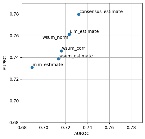
It looks like mlm this time had worse performance than other methods like ulm at recovering perturbed regulators, this might be caused because there are many TFs that share too many targets. Whenever there are multiple sources (TFs) and they share a lot of targets we recommend to use ulm. On the other hand, when there are few sources and they are orthogonal (they share few targets), we recommend to use mlm. Since consensus remains one of the top performer methods we also recommend its use but at a higher computational cost and less interpretability.

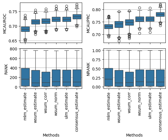
We can also visualise the distirbutions of the obtained metrics, for example mcauroc, mcauprc, rank and nrank:

fig, axes = plt.subplots(2, 2, figsize=(6, 5), sharex=True, tight_layout=True)
dc.plot_metrics_boxplot(df, metric='mcauroc', ax=axes[0, 0])
dc.plot_metrics_boxplot(df, metric='mcauprc', ax=axes[0, 1])
dc.plot_metrics_boxplot(df, metric='rank', ax=axes[1, 0])
dc.plot_metrics_boxplot(df, metric='nrank', ax=axes[1, 1])

Multiple networks

This pipeline can evaluate multiple networks at the same time. Now we will evaluate CollecTRI and DoRothEA, a literature-based network that we developed in the past. We will also add a randomized version as control.

# Get dorothea
dorothea = dc.get_dorothea(organism='human')

# Randomize nets
ctri_rand = dc.shuffle_net(collectri, target='target', weight='weight').drop_duplicates(['source', 'target'])
doro_rand = dc.shuffle_net(dorothea, target='target', weight='weight').drop_duplicates(['source', 'target'])

We can run the same pipeline but now using a dictionary of networks (and of extra arguments if needed).

# Build dictionary of networks to test
nets = {
    'r_collectri': ctri_rand,
    'r_dorothea': doro_rand,
    'collectri': collectri,
    'dorothea': dorothea,
}

# Example extra arguments
decouple_kws = {
    'r_collectri': {
        'methods' : ['ulm', 'mlm'],
        'consensus': True
    },
    'r_dorothea': {
        'methods' : ['ulm', 'mlm'],
        'consensus': True
    },
    'collectri': {
        'methods' : ['ulm', 'mlm'],
        'consensus': True
    },
    'dorothea': {
        'methods' : ['ulm', 'mlm'],
        'consensus': True
    }
}

# Run benchmark pipeline
df = dc.benchmark(mat, obs, nets, perturb='TF', sign=-1, verbose=True, decouple_kws=decouple_kws)

Using r_collectri network...
Extracting inputs...
Formating net...
Removed 109 experiments without sources in net.
Running 279 experiments for 155 unique sources.
Running methods...
52 features of mat are empty, they will be removed.
Running ulm on mat with 279 samples and 21933 targets for 762 sources.
52 features of mat are empty, they will be removed.
Running mlm on mat with 279 samples and 21933 targets for 762 sources.
Calculating metrics...
Computing metrics...
Done.
Using r_dorothea network...
Extracting inputs...
Formating net...
Removed 175 experiments without sources in net.
Running 213 experiments for 104 unique sources.
Running methods...
55 features of mat are empty, they will be removed.
Running ulm on mat with 213 samples and 21930 targets for 295 sources.
55 features of mat are empty, they will be removed.
Running mlm on mat with 213 samples and 21930 targets for 295 sources.
Calculating metrics...
Computing metrics...
Done.
Using collectri network...
Extracting inputs...
Formating net...
Removed 109 experiments without sources in net.
Running 279 experiments for 155 unique sources.
Running methods...
52 features of mat are empty, they will be removed.
Running ulm on mat with 279 samples and 21933 targets for 766 sources.
52 features of mat are empty, they will be removed.
Running mlm on mat with 279 samples and 21933 targets for 766 sources.
Calculating metrics...
Computing metrics...
Done.
Using dorothea network...
Extracting inputs...
Formating net...
Removed 174 experiments without sources in net.
Running 214 experiments for 105 unique sources.
Running methods...
55 features of mat are empty, they will be removed.
Running ulm on mat with 214 samples and 21930 targets for 297 sources.
55 features of mat are empty, they will be removed.
Running mlm on mat with 214 samples and 21930 targets for 297 sources.
Calculating metrics...
Computing metrics...
Done.

Like before we can try to visualize the results in a scatterplot, this time grouping by the network used:

dc.plot_metrics_scatter(df, groupby='net', x='mcauroc', y='mcauprc')

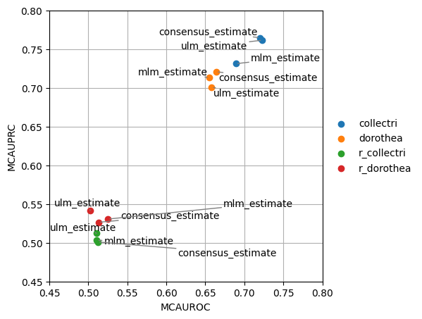
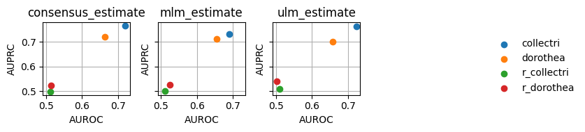
Since this plot is too crowded, we can plot it again separating the methods by columns:

dc.plot_metrics_scatter_cols(df, col='method', x='auroc', y='auprc', figsize=(7, 2), groupby='net')

Or by selecting only one of the methods, in this case consensus:

dc.plot_metrics_scatter(df[df['method'] == 'consensus_estimate'], groupby='net', x='mcauroc', y='mcauprc', show_text=False, figsize=(2, 2))

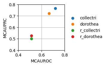
As expected, the random network has a performance close to 0.5 while the rest show higher predictive performance. As previously reported, the collectri network has better performance than dorothea.

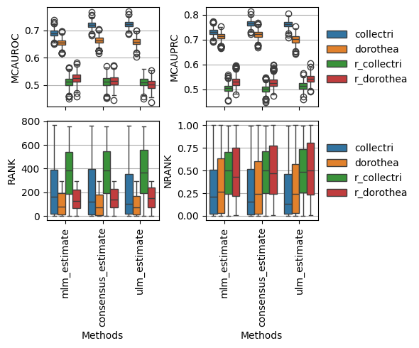
If needed, we can also plot the distributions of the Monte-Carlo metrics, now grouped by network:

fig, axes = plt.subplots(2, 2, figsize=(6, 5), sharex=True, tight_layout=True)
dc.plot_metrics_boxplot(df, metric='mcauroc', groupby='net', ax=axes[0, 0], legend=False)
dc.plot_metrics_boxplot(df, metric='mcauprc', groupby='net', ax=axes[0, 1], legend=True)
dc.plot_metrics_boxplot(df, metric='rank', groupby='net', ax=axes[1, 0], legend=False)
dc.plot_metrics_boxplot(df, metric='nrank', groupby='net', ax=axes[1, 1])

By source

The benchmark pipeline also allows to test the performance of individual regulators using the argument by='source'. For simplicity let us just use the best performing network:

# Example on how to set up decouple arguments
decouple_kws={
    'methods' : ['ulm', 'mlm'],
    'consensus': True,
}

# Run benchmark pipeline
df = dc.benchmark(mat, obs, collectri, perturb='TF', sign=-1, by='source', verbose=True, decouple_kws=decouple_kws)

Extracting inputs...
Formating net...
Removed 109 experiments without sources in net.
Running 279 experiments for 155 unique sources.
Running methods...
52 features of mat are empty, they will be removed.
Running ulm on mat with 279 samples and 21933 targets for 766 sources.
52 features of mat are empty, they will be removed.
Running mlm on mat with 279 samples and 21933 targets for 766 sources.
Calculating metrics...
Computing metrics...
Done.

We can plot the results with:

dc.plot_metrics_scatter_cols(df, col='source', figsize=(6, 5), groupby='method')

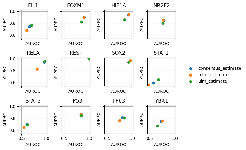
It looks like we get good predictions for HIF1A, RELA and SOX2 among others. On the other side, we worse predictions for STAT1.

By meta-data groups

The benchmarking pipeline can also be run by grouping the input experiments using the groupby argument. Multiple groups can be selected at the same time but for simplicity, we will just test which knockout method seems to perform the best inhibitions:

# Example on how to set up decouple arguments
decouple_kws={
    'methods' : ['ulm', 'mlm'],
    'consensus': True,
}

# Run benchmark pipeline
df = dc.benchmark(mat, obs, collectri, perturb='TF', sign=-1, groupby='Knock.Method', verbose=True, decouple_kws=decouple_kws)

Extracting inputs...
Formating net...
Removed 109 experiments without sources in net.
Running 279 experiments for 155 unique sources.
Running methods...
52 features of mat are empty, they will be removed.
Running ulm on mat with 279 samples and 21933 targets for 766 sources.
52 features of mat are empty, they will be removed.
Running mlm on mat with 279 samples and 21933 targets for 766 sources.
Calculating metrics...
Computing metrics for groupby Knock.Method...
Done.

Again, we can visualize the results in a collection of scatterplots:

dc.plot_metrics_scatter_cols(df, col='method', figsize=(7, 2), groupby='group')

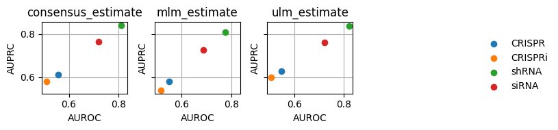
From our limited data-set, we can see that apparently shRNA works better than other knockout protocols.