Functional enrichment of biological terms
scRNA-seq yield many molecular readouts that are hard to interpret by themselves. One way of summarizing this information is by assigning them to biological terms from prior knowledge.
In this notebook we showcase how to use decoupler for functional enrichment with the 3k PBMCs 10X data-set. The data consists of 3k PBMCs from a Healthy Donor and is freely available from 10x Genomics here from this webpage
Note
This tutorial assumes that you already know the basics of decoupler. Else, check out the Usage tutorial first.
Loading packages
First, we need to load the relevant packages, scanpy to handle scRNA-seq data and decoupler to use statistical methods.
[1]:
import scanpy as sc
import decoupler as dc
import numpy as np

# Plotting options, change to your liking
sc.settings.set_figure_params(dpi=200, frameon=False)
sc.set_figure_params(dpi=200)
sc.set_figure_params(figsize=(4, 4))
Loading the data
We can download the data easily using scanpy:
[2]:
adata = sc.datasets.pbmc3k_processed()
adata
[2]:
AnnData object with n_obs × n_vars = 2638 × 1838
    obs: 'n_genes', 'percent_mito', 'n_counts', 'louvain'
    var: 'n_cells'
    uns: 'draw_graph', 'louvain', 'louvain_colors', 'neighbors', 'pca', 'rank_genes_groups'
    obsm: 'X_pca', 'X_tsne', 'X_umap', 'X_draw_graph_fr'
    varm: 'PCs'
    obsp: 'distances', 'connectivities'
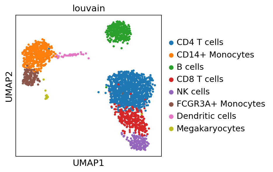
We can visualize the different cell types in it:
[3]:
sc.pl.umap(adata, color='louvain')
MSigDB gene sets
The Molecular Signatures Database (MSigDB) is a resource containing a collection of gene sets annotated to different biological processes.
[4]:
msigdb = dc.get_resource('MSigDB')
msigdb
[4]:
| genesymbol | collection | geneset | |
|---|---|---|---|
| 0 | MAFF | chemical_and_genetic_perturbations | BOYAULT_LIVER_CANCER_SUBCLASS_G56_DN |
| 1 | MAFF | chemical_and_genetic_perturbations | ELVIDGE_HYPOXIA_UP |
| 2 | MAFF | chemical_and_genetic_perturbations | NUYTTEN_NIPP1_TARGETS_DN |
| 3 | MAFF | immunesigdb | GSE17721_POLYIC_VS_GARDIQUIMOD_4H_BMDC_DN |
| 4 | MAFF | chemical_and_genetic_perturbations | SCHAEFFER_PROSTATE_DEVELOPMENT_12HR_UP |
| ... | ... | ... | ... |
| 3838543 | PRAMEF22 | go_biological_process | GOBP_POSITIVE_REGULATION_OF_CELL_POPULATION_PR... |
| 3838544 | PRAMEF22 | go_biological_process | GOBP_APOPTOTIC_PROCESS |
| 3838545 | PRAMEF22 | go_biological_process | GOBP_REGULATION_OF_CELL_DEATH |
| 3838546 | PRAMEF22 | go_biological_process | GOBP_NEGATIVE_REGULATION_OF_DEVELOPMENTAL_PROCESS |
| 3838547 | PRAMEF22 | go_biological_process | GOBP_NEGATIVE_REGULATION_OF_CELL_DEATH |
3838548 rows × 3 columns
As an example, we will use the hallmark gene sets, but we could have used any other such as KEGG or REACTOME.
Note
To see what other collections are available in MSigDB, type: msigdb['collection'].unique().
We can filter by for hallmark:
[5]:
# Filter by hallmark
msigdb = msigdb[msigdb['collection']=='hallmark']

# Remove duplicated entries
msigdb = msigdb[~msigdb.duplicated(['geneset', 'genesymbol'])]
msigdb
[5]:
| genesymbol | collection | geneset | |
|---|---|---|---|
| 233 | MAFF | hallmark | HALLMARK_IL2_STAT5_SIGNALING |
| 250 | MAFF | hallmark | HALLMARK_COAGULATION |
| 270 | MAFF | hallmark | HALLMARK_HYPOXIA |
| 373 | MAFF | hallmark | HALLMARK_TNFA_SIGNALING_VIA_NFKB |
| 377 | MAFF | hallmark | HALLMARK_COMPLEMENT |
| ... | ... | ... | ... |
| 1449668 | STXBP1 | hallmark | HALLMARK_PANCREAS_BETA_CELLS |
| 1450315 | ELP4 | hallmark | HALLMARK_PANCREAS_BETA_CELLS |
| 1450526 | GCG | hallmark | HALLMARK_PANCREAS_BETA_CELLS |
| 1450731 | PCSK2 | hallmark | HALLMARK_PANCREAS_BETA_CELLS |
| 1450916 | PAX6 | hallmark | HALLMARK_PANCREAS_BETA_CELLS |
7318 rows × 3 columns
For this example we will use the resource MSigDB, but we could have used any other such as GO. To see the list of available resources inside Omnipath, run dc.show_resources()
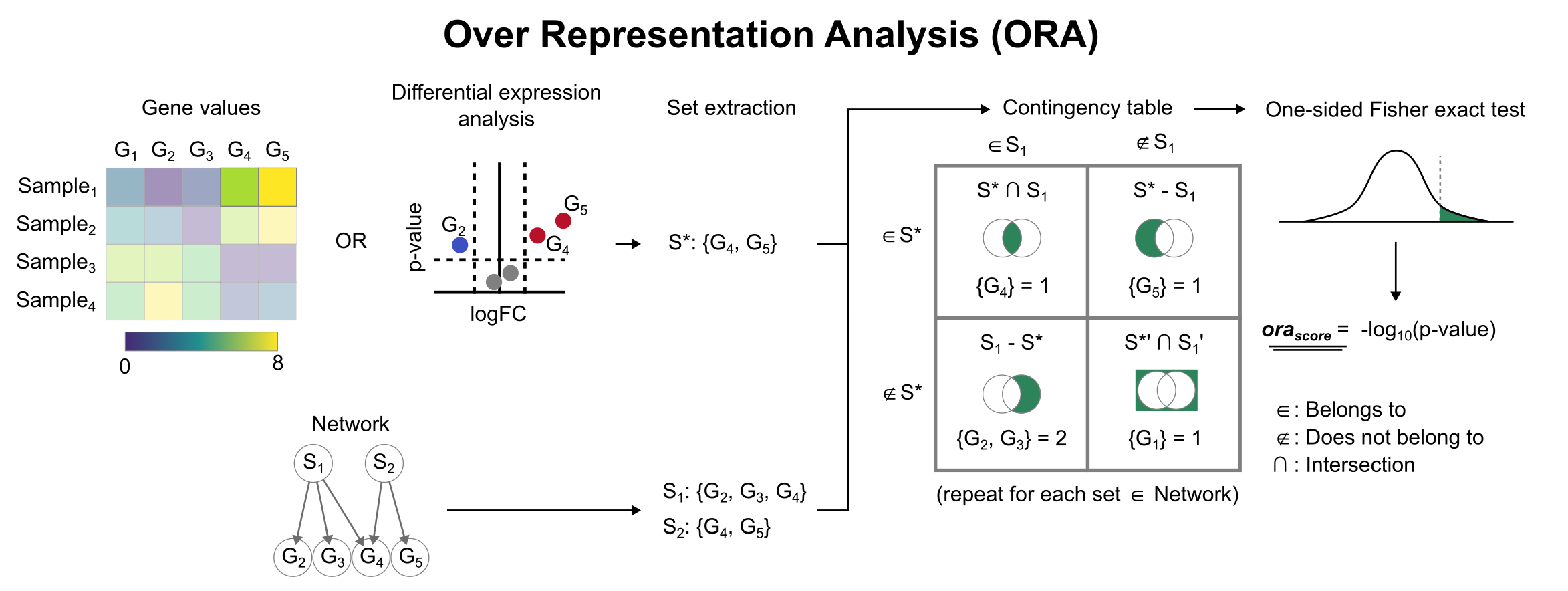
Enrichment with Over Representation Analysis (ORA)
To infer functional enrichment scores we will run the Over Representation Analysis (ora) method. As input data it accepts an expression matrix (decoupler.run_ora) or the results of differential expression analysis (decoupler.run_ora_df). For the former, by default the top 5% of expressed genes by sample are selected as the set of interest (S), and for the latter a user-defined significance filtering can be used. Once we have S, it builds a contingency table using set operations
for each set stored in the gene set resource being used (net). Using the contingency table, ora performs a one-sided Fisher exact test to test for significance of overlap between sets. The final score is obtained by log-transforming the obtained p-values, meaning that higher values are more significant.
We can run ora with a simple one-liner:
[6]:
dc.run_ora(
    mat=adata,
    net=msigdb,
    source='geneset',
    target='genesymbol',
    verbose=True
)
1 features of mat are empty, they will be removed.
Running ora on mat with 2638 samples and 13713 targets for 50 sources.
100%|████████████████████████████████████████████████████████████████████████████████████████████████████████████████████| 2638/2638 [00:02<00:00, 919.66it/s]
The obtained scores (-log10(p-value))(ora_estimate) and p-values (ora_pvals) are stored in the .obsm key:
[7]:
adata.obsm['ora_estimate']
[7]:
| source | HALLMARK_ADIPOGENESIS | HALLMARK_ALLOGRAFT_REJECTION | HALLMARK_ANDROGEN_RESPONSE | HALLMARK_ANGIOGENESIS | HALLMARK_APICAL_JUNCTION | HALLMARK_APICAL_SURFACE | HALLMARK_APOPTOSIS | HALLMARK_BILE_ACID_METABOLISM | HALLMARK_CHOLESTEROL_HOMEOSTASIS | HALLMARK_COAGULATION | ... | HALLMARK_PROTEIN_SECRETION | HALLMARK_REACTIVE_OXYGEN_SPECIES_PATHWAY | HALLMARK_SPERMATOGENESIS | HALLMARK_TGF_BETA_SIGNALING | HALLMARK_TNFA_SIGNALING_VIA_NFKB | HALLMARK_UNFOLDED_PROTEIN_RESPONSE | HALLMARK_UV_RESPONSE_DN | HALLMARK_UV_RESPONSE_UP | HALLMARK_WNT_BETA_CATENIN_SIGNALING | HALLMARK_XENOBIOTIC_METABOLISM |
|---|---|---|---|---|---|---|---|---|---|---|---|---|---|---|---|---|---|---|---|---|---|
| AAACATACAACCAC-1 | 1.307006 | 10.029702 | 0.822139 | 0.389675 | 1.670031 | 0.650245 | 2.441094 | 0.337563 | 0.805206 | 0.032740 | ... | 0.733962 | 2.286568 | 0.354931 | 2.986336 | 8.270970 | 6.424740 | 0.586324 | 1.983873 | 0.164805 | 0.080157 |
| AAACATTGAGCTAC-1 | 1.307006 | 14.824231 | 2.152116 | 0.389675 | 2.104104 | -0.000000 | 0.442704 | 0.337563 | 0.457516 | 0.321093 | ... | 2.496213 | 1.659624 | 1.015676 | 1.659624 | 3.053600 | 2.578916 | 0.346751 | 0.871448 | 0.503794 | 0.080157 |
| AAACATTGATCAGC-1 | 3.893118 | 7.893567 | 3.312021 | 0.389675 | 3.095283 | 0.650245 | 5.115631 | 0.976973 | 0.805206 | 0.321093 | ... | 1.087271 | 3.752012 | 0.037885 | 1.114303 | 7.597478 | 2.075696 | 0.888675 | 4.038435 | 0.164805 | 1.087420 |
| AAACCGTGCTTCCG-1 | 5.591584 | 7.893567 | 2.152116 | 1.036748 | 1.670031 | -0.000000 | 2.911700 | 0.143019 | 1.747025 | 0.591452 | ... | 1.501986 | 3.752012 | 0.354931 | 1.659624 | 5.709134 | 5.000056 | 0.346751 | 1.567924 | 0.164805 | 1.087420 |
| AAACCGTGTATGCG-1 | 0.999733 | 10.029702 | 2.707608 | 1.871866 | 1.670031 | 1.948869 | 0.666121 | 0.337563 | 0.805206 | 0.591452 | ... | 1.973108 | 1.659624 | 0.151790 | 1.114303 | 1.803915 | 1.212284 | 0.586324 | 0.375221 | 0.164805 | 0.179270 |
| ... | ... | ... | ... | ... | ... | ... | ... | ... | ... | ... | ... | ... | ... | ... | ... | ... | ... | ... | ... | ... | ... |
| TTTCGAACTCTCAT-1 | 3.382339 | 9.297059 | 1.204403 | 1.036748 | 2.580035 | 0.224257 | 10.804691 | 0.143019 | 2.324194 | 1.359530 | ... | 3.683543 | 3.752012 | 0.151790 | 2.286568 | 5.709134 | 2.075696 | 0.586324 | 4.639190 | 0.164805 | 1.087420 |
| TTTCTACTGAGGCA-1 | 6.851412 | 4.777953 | 6.964458 | 1.036748 | 1.670031 | 0.650245 | 2.006126 | 0.035215 | 0.457516 | 1.359530 | ... | 3.683543 | 1.659624 | 0.151790 | 2.286568 | 2.188676 | 8.792837 | 0.172992 | 2.441252 | 0.164805 | 0.080157 |
| TTTCTACTTCCTCG-1 | 1.652714 | 7.224005 | 2.152116 | -0.000000 | 1.670031 | 1.235034 | 2.441094 | 0.337563 | 1.238111 | 0.134773 | ... | 1.087271 | 0.661862 | 0.151790 | 1.659624 | 8.965328 | 3.125529 | 0.064563 | 4.639190 | -0.000000 | 0.329247 |
| TTTGCATGAGAGGC-1 | 2.034900 | 5.352930 | 1.204403 | 1.036748 | 0.939005 | 1.235034 | 0.267770 | 0.617706 | 0.805206 | 0.134773 | ... | 0.733962 | 2.286568 | 0.151790 | 0.661862 | 3.530830 | 5.696068 | 0.346751 | 2.441252 | 0.164805 | 0.329247 |
| TTTGCATGCCTCAC-1 | 1.307006 | 10.029702 | 0.508632 | 0.389675 | 1.670031 | 0.650245 | 3.416073 | 0.976973 | 0.457516 | 0.134773 | ... | 0.232568 | 2.286568 | 0.037885 | 1.659624 | 3.530830 | 5.000056 | 0.888675 | 4.038435 | 0.164805 | 0.080157 |
2638 rows × 50 columns
Visualization
To visualize the obtianed scores, we can re-use many of scanpy’s plotting functions. First though, we need to extract them from the adata object.
[8]:
acts = dc.get_acts(adata, obsm_key='ora_estimate')

# We need to remove inf and set them to the maximum value observed
acts_v = acts.X.ravel()
max_e = np.nanmax(acts_v[np.isfinite(acts_v)])
acts.X[~np.isfinite(acts.X)] = max_e

acts
[8]:
AnnData object with n_obs × n_vars = 2638 × 50
    obs: 'n_genes', 'percent_mito', 'n_counts', 'louvain'
    uns: 'draw_graph', 'louvain', 'louvain_colors', 'neighbors', 'pca', 'rank_genes_groups'
    obsm: 'X_pca', 'X_tsne', 'X_umap', 'X_draw_graph_fr', 'ora_estimate', 'ora_pvals'
dc.get_acts returns a new AnnData object which holds the obtained activities in its .X attribute, allowing us to re-use many scanpy functions, for example:
[9]:
sc.pl.umap(acts, color=['HALLMARK_COAGULATION', 'louvain'], cmap='RdBu_r')
sc.pl.violin(acts, keys=['HALLMARK_COAGULATION'], groupby='louvain', rotation=90)
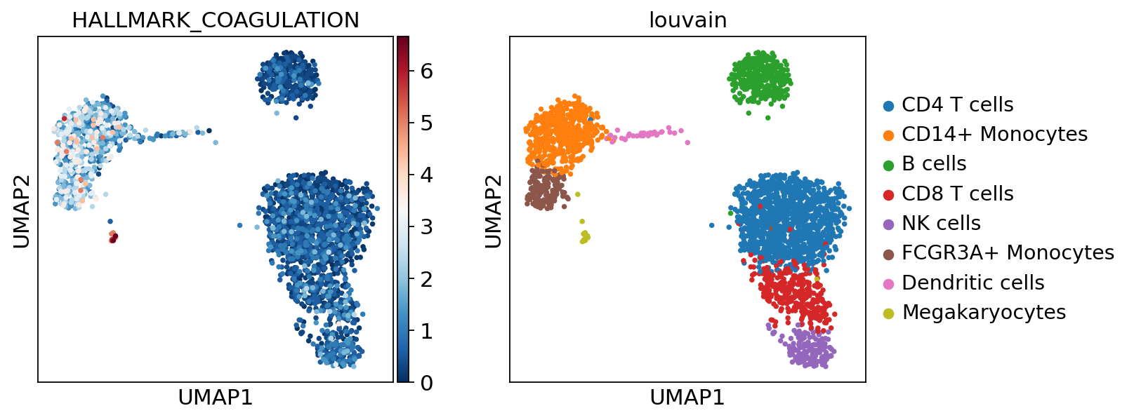
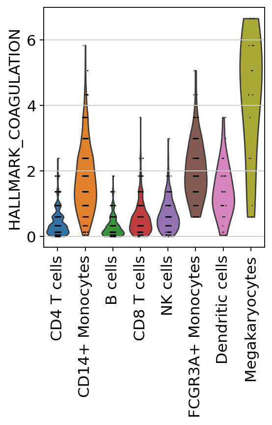
The cells highlighted seem to be enriched by coagulation.
Exploration
Let’s identify which are the top gene sets per cell type. We can do it by using the function dc.rank_sources_groups, which identifies marker gene sets using the same statistical tests available in scanpy’s scanpy.tl.rank_genes_groups.
[10]:
df = dc.rank_sources_groups(acts, groupby='louvain', reference='rest', method='t-test_overestim_var')
df
[10]:
| group | reference | names | statistic | meanchange | pvals | pvals_adj | |
|---|---|---|---|---|---|---|---|
| 0 | B cells | rest | HALLMARK_KRAS_SIGNALING_DN | 8.300668 | 0.171902 | 6.620000e-16 | 3.009091e-15 |
| 1 | B cells | rest | HALLMARK_HEDGEHOG_SIGNALING | 2.108226 | 0.027850 | 3.538195e-02 | 5.528430e-02 |
| 2 | B cells | rest | HALLMARK_MYOGENESIS | 1.896726 | 0.074938 | 5.829358e-02 | 8.327655e-02 |
| 3 | B cells | rest | HALLMARK_ALLOGRAFT_REJECTION | 0.968864 | 0.204067 | 3.329577e-01 | 4.161971e-01 |
| 4 | B cells | rest | HALLMARK_SPERMATOGENESIS | 0.521071 | 0.009809 | 6.024869e-01 | 6.846442e-01 |
| ... | ... | ... | ... | ... | ... | ... | ... |
| 395 | NK cells | rest | HALLMARK_REACTIVE_OXYGEN_SPECIES_PATHWAY | -3.210821 | -0.487032 | 1.466372e-03 | 6.109882e-03 |
| 396 | NK cells | rest | HALLMARK_UV_RESPONSE_UP | -3.215664 | -0.479964 | 1.447535e-03 | 6.109882e-03 |
| 397 | NK cells | rest | HALLMARK_ANGIOGENESIS | -3.911384 | -0.256110 | 1.214908e-04 | 8.677915e-04 |
| 398 | NK cells | rest | HALLMARK_IL6_JAK_STAT3_SIGNALING | -4.133565 | -0.324985 | 4.637187e-05 | 3.864322e-04 |
| 399 | NK cells | rest | HALLMARK_TNFA_SIGNALING_VIA_NFKB | -5.326771 | -1.326010 | 2.021269e-07 | 5.053172e-06 |
400 rows × 7 columns
We can then extract the top 3 markers per cell type:
[11]:
n_markers = 3
source_markers = df.groupby('group').head(n_markers).groupby('group')['names'].apply(lambda x: list(x)).to_dict()
source_markers
[11]:
{'B cells': ['HALLMARK_KRAS_SIGNALING_DN',
  'HALLMARK_HEDGEHOG_SIGNALING',
  'HALLMARK_MYOGENESIS'],
 'CD14+ Monocytes': ['HALLMARK_COMPLEMENT',
  'HALLMARK_COAGULATION',
  'HALLMARK_EPITHELIAL_MESENCHYMAL_TRANSITION'],
 'CD4 T cells': ['HALLMARK_WNT_BETA_CATENIN_SIGNALING',
  'HALLMARK_MYC_TARGETS_V1',
  'HALLMARK_MYC_TARGETS_V2'],
 'CD8 T cells': ['HALLMARK_ALLOGRAFT_REJECTION',
  'HALLMARK_MYC_TARGETS_V2',
  'HALLMARK_PI3K_AKT_MTOR_SIGNALING'],
 'Dendritic cells': ['HALLMARK_OXIDATIVE_PHOSPHORYLATION',
  'HALLMARK_MYC_TARGETS_V1',
  'HALLMARK_ALLOGRAFT_REJECTION'],
 'FCGR3A+ Monocytes': ['HALLMARK_COMPLEMENT',
  'HALLMARK_COAGULATION',
  'HALLMARK_INTERFERON_GAMMA_RESPONSE'],
 'Megakaryocytes': ['HALLMARK_COAGULATION',
  'HALLMARK_ANGIOGENESIS',
  'HALLMARK_MYOGENESIS'],
 'NK cells': ['HALLMARK_ALLOGRAFT_REJECTION',
  'HALLMARK_INTERFERON_GAMMA_RESPONSE',
  'HALLMARK_INTERFERON_ALPHA_RESPONSE']}
We can plot the obtained markers:
[12]:
sc.pl.matrixplot(acts, source_markers, 'louvain', dendrogram=True, standard_scale='var',
                 colorbar_title='Z-scaled scores', cmap='RdBu_r')
WARNING: dendrogram data not found (using key=dendrogram_louvain). Running `sc.tl.dendrogram` with default parameters. For fine tuning it is recommended to run `sc.tl.dendrogram` independently.
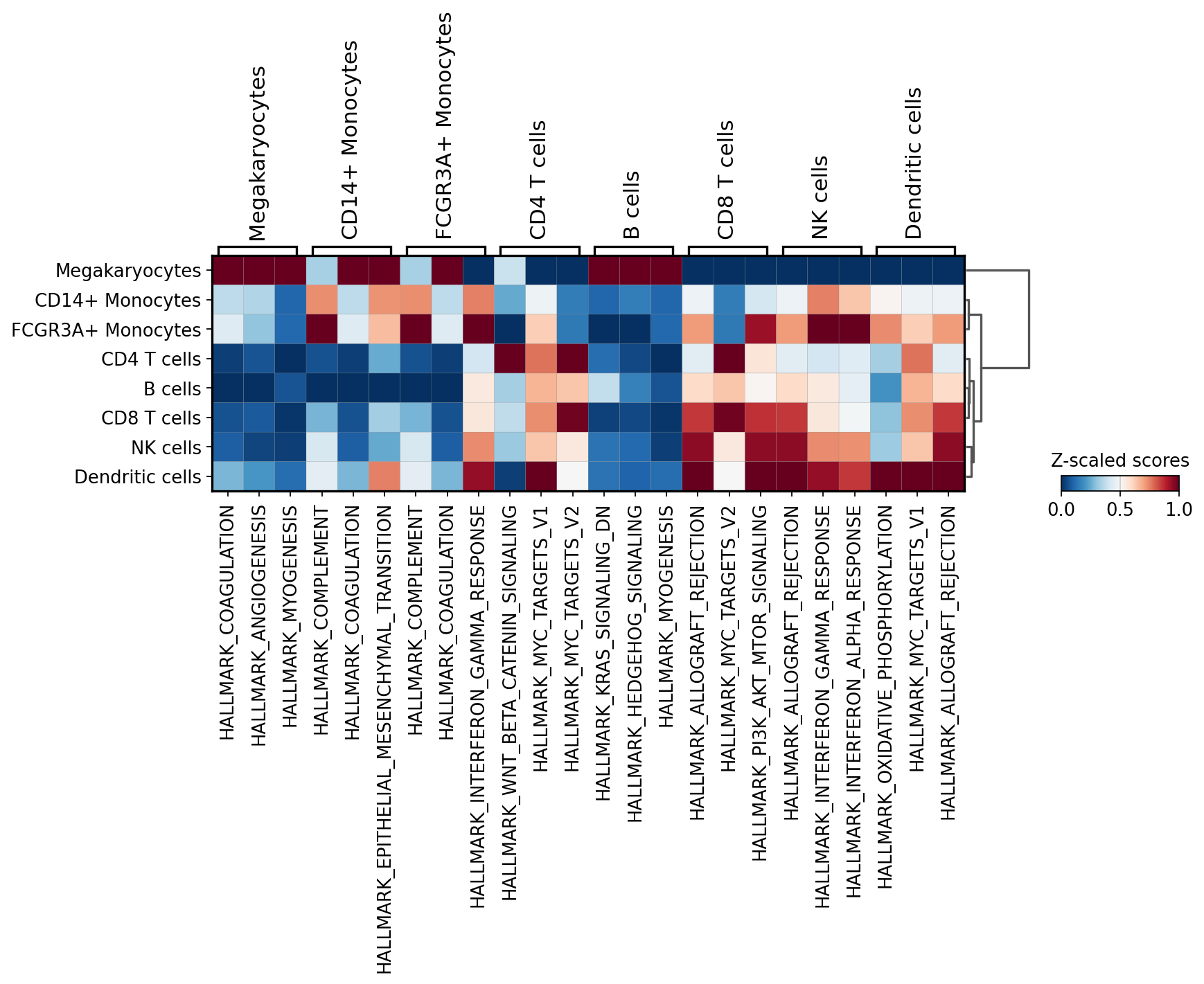
In this specific example, we can observe that myeloid cell types are enriched by the complement’s system genes and megakaryocytes are enriched by coagulation genes.
Note
If your data consist of different conditions with enough samples, we recommend to work with pseudo-bulk profiles instead. Check this vignette for more informatin.