Transcription factor activity inference

scRNA-seq yield many molecular readouts that are hard to interpret by themselves. One way of summarizing this information is by infering transcription factor (TF) activities from prior knowledge.

In this notebook we showcase how to use decoupler for TF activity inference with the 3k PBMCs 10X data-set. The data consists of 3k PBMCs from a Healthy Donor and is freely available from 10x Genomics here from this webpage

Note

This tutorial assumes that you already know the basics of decoupler. Else, check out the Usage tutorial first.

Loading packages

First, we need to load the relevant packages, scanpy to handle scRNA-seq data and decoupler to use statistical methods.

[1]:

import scanpy as sc
import decoupler as dc

# Only needed for visualization:
import matplotlib.pyplot as plt
import seaborn as sns

Loading the data

We can download the data easily using scanpy:

[2]:

adata = sc.datasets.pbmc3k_processed()
adata

[2]:

AnnData object with n_obs × n_vars = 2638 × 1838
    obs: 'n_genes', 'percent_mito', 'n_counts', 'louvain'
    var: 'n_cells'
    uns: 'draw_graph', 'louvain', 'louvain_colors', 'neighbors', 'pca', 'rank_genes_groups'
    obsm: 'X_pca', 'X_tsne', 'X_umap', 'X_draw_graph_fr'
    varm: 'PCs'
    obsp: 'distances', 'connectivities'

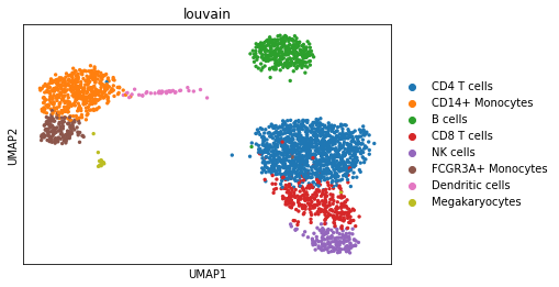
We can visualize the different cell types in it:

[3]:

sc.pl.umap(adata, color='louvain')

DoRothEA network

DoRothEA is a comprehensive resource containing a curated collection of TFs and their transcriptional targets. Since these regulons were gathered from different types of evidence, interactions in DoRothEA are classified in different confidence levels, ranging from A (highest confidence) to D (lowest confidence). Moreover, each interaction is weighted by its confidence level and the sign of its mode of regulation (activation or inhibition).

For this example we will use the human version (mouse is also available) and we will use the confidence levels ABC. To access it we can use decoupler.

[4]:

net = dc.get_dorothea(organism='human', levels=['A','B','C'])
net

[4]:

	source	confidence	target	weight
32	ADNP	C	ATF7IP	0.333333
99	ADNP	C	DYRK1A	0.333333
325	ADNP	C	TLK1	0.333333
355	ADNP	C	ZMYM4	0.333333
383	AHR	C	ARHGAP15	0.333333
...	...	...	...	...
277557	ZNF766	C	MARF1	0.333333
277760	ZNF83	C	CUBN	0.333333
277842	ZNF83	C	PCBP1	0.333333
277885	ZNF83	C	SND1	0.333333
277920	ZNF83	C	ZNF331	0.333333

32277 rows × 4 columns

Activity inference with Multivariate Linear Model

To infer activities we will run the Multivariate Linear Model method (mlm). It models the observed gene expression by using a regulatory adjacency matrix (target genes x TFs) as covariates of a linear model. The values of this matrix are the associated interaction weights. The obtained t-values of the fitted model are the activity scores.

To run decoupler methods, we need an input matrix (mat), an input prior knowledge network/resource (net), and the name of the columns of net that we want to use.

[5]:

dc.run_mlm(mat=adata, net=net, source='source', target='target', weight='weight', verbose=True)

58 features of mat are empty in 2635 samples, they will be ignored.
Running mlm on mat with 2638 samples and 13656 targets for 281 sources.

100%|██████████████████████████████████████████████████████████████████████████████████████████████████████████████████████████████████████| 1/1 [00:02<00:00,  2.69s/it]

The obtained scores (t-values)(mlm_estimate) and p-values (mlm_pvals) are stored in the .obsm key:

[6]:

adata.obsm['mlm_estimate']

[6]:

	AHR	AR	ARID2	ARID3A	ARNT	ARNTL	ASCL1	ATF1	ATF2	ATF3	...	ZNF217	ZNF24	ZNF263	ZNF274	ZNF384	ZNF584	ZNF592	ZNF639	ZNF644	ZNF740
AAACATACAACCAC-1	1.378135	2.264273	-0.873322	-0.393858	0.138300	-0.672718	-0.517479	-0.248986	3.503265	2.835963	...	0.184587	-0.368374	-2.079961	-0.819101	-1.070376	-0.513939	-0.168147	1.016369	-0.426693	0.321183
AAACATTGAGCTAC-1	-0.771592	1.791025	-0.843771	-2.423655	1.121631	-1.710017	-0.098786	-0.437355	1.153930	0.325601	...	0.975836	-1.015507	-1.298664	-0.695452	-0.717216	-0.854899	-0.634035	-0.014624	0.189121	0.082495
AAACATTGATCAGC-1	1.692710	2.992034	-0.532615	-1.705098	0.845731	-1.167016	-0.788160	1.828757	3.575169	2.071486	...	0.001384	-0.424543	-2.065581	-0.535091	-0.751262	0.057934	0.295792	1.095627	1.089436	1.264037
AAACCGTGCTTCCG-1	0.950064	2.362731	-0.064999	-2.908230	0.925053	-1.022329	-0.007307	0.157366	2.790008	0.088670	...	0.729664	-0.744951	-1.341359	-1.054481	-1.698370	-0.830679	-0.641169	-0.139106	-0.632336	-0.595452
AAACCGTGTATGCG-1	1.064581	1.690591	-0.638252	-1.559646	0.021609	-1.933049	-0.375894	-1.909076	-2.098804	2.609869	...	1.399544	-0.788018	-1.914087	0.276000	-0.631482	-0.596122	0.775489	0.925926	-0.350876	0.218557
...	...	...	...	...	...	...	...	...	...	...	...	...	...	...	...	...	...	...	...	...	...
TTTCGAACTCTCAT-1	0.318688	3.333595	-0.411664	-1.804654	-0.024565	-1.428001	-0.363318	-0.074915	1.548303	-1.499557	...	0.924372	0.169212	-1.506868	-1.248334	-0.712812	-0.823596	-0.452081	-0.257280	0.458884	-0.125251
TTTCTACTGAGGCA-1	0.030770	3.491437	-0.003791	-1.533359	1.548976	-1.666779	-0.371404	0.731910	2.437067	-0.304436	...	0.801202	-0.535329	-1.734694	-0.584308	-1.229465	-1.455734	0.495586	1.191117	-0.316089	-0.160711
TTTCTACTTCCTCG-1	0.832445	1.216446	-0.077293	-2.480361	1.021587	-1.059844	-0.543997	0.110234	4.672308	0.357114	...	0.063306	-0.711501	-0.494086	-0.123922	0.307080	-0.587546	-0.336605	-0.489180	-0.105757	0.136211
TTTGCATGAGAGGC-1	1.639155	-1.020706	-0.213240	-1.343566	-1.097421	-1.058532	-0.473836	-1.477254	3.461115	-0.166357	...	0.090237	-0.554044	-1.828985	-0.717352	-1.356452	0.781485	-0.567864	1.205502	-0.513317	-0.485571
TTTGCATGCCTCAC-1	0.603490	1.357359	-0.001079	-0.808231	0.574937	-0.918280	0.057767	-0.138379	3.882482	0.035893	...	0.123596	-0.818702	-1.486360	-0.168504	-0.349759	-0.609642	-0.524824	0.367838	-0.639741	-1.074070

2638 rows × 281 columns

Visualization

To visualize the obtained scores, we can re-use many of scanpy’s plotting functions. First though, we need to extract them from the adata object.

[7]:

acts = dc.get_acts(adata, obsm_key='mlm_estimate')
acts

[7]:

AnnData object with n_obs × n_vars = 2638 × 281
    obs: 'n_genes', 'percent_mito', 'n_counts', 'louvain'
    uns: 'draw_graph', 'louvain', 'louvain_colors', 'neighbors', 'pca', 'rank_genes_groups'
    obsm: 'X_pca', 'X_tsne', 'X_umap', 'X_draw_graph_fr', 'mlm_estimate', 'mlm_pvals'

dc.get_acts returns a new AnnData object which holds the obtained activities in its .X attribute, allowing us to re-use many scanpy functions, for example:

[8]:

sc.pl.umap(acts, color=['PAX5', 'louvain'], cmap='coolwarm', vcenter=0)

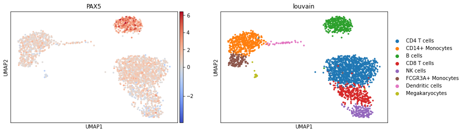
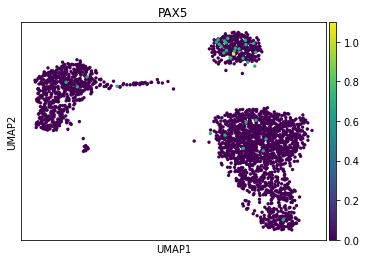
Here we observe the activity infered for PAX5 across cells, which it is particulary active in B cells. Interestingly, PAX5 is a known TF crucial for B cell identity and function. The inference of activities from “foot-prints” of target genes is more informative than just looking at the molecular readouts of a given TF, as an example here is the gene expression of PAX5, which is not very informative by itself:

[9]:

sc.pl.umap(adata, color='PAX5')

Exploration

With decoupler we can also see what is the mean activity per group:

[10]:

mean_acts = dc.summarize_acts(acts, groupby='louvain', min_std=0.75)
mean_acts

[10]:

	ATF2	ATF3	BACH2	CEBPB	CREB1	CREM	E2F7	ELK1	ESR2	FLI1	...	REL	RFX5	SPI1	SRF	STAT3	STAT4	TWIST1	USF2	VDR	ZEB2
B cells	2.862969	0.019417	1.465132	-1.228275	0.766851	-1.464812	2.403033	2.052581	3.010641	-1.225937	...	-0.235809	13.664467	1.983899	1.009392	0.446212	-0.634330	-0.379897	1.135778	3.559175	1.004979
CD14+ Monocytes	1.999015	0.171993	2.853407	0.873314	-1.068738	-1.807258	3.214978	1.698306	5.127353	-0.795042	...	-0.484027	6.790155	3.596492	2.012946	1.400468	2.490378	-0.830065	0.463730	3.634538	2.253694
CD4 T cells	2.803929	0.874975	1.300077	-1.456407	-0.922025	-1.801688	2.631588	2.954413	3.755870	-0.997119	...	-0.048043	1.297521	1.478310	1.341560	1.228789	0.390740	-0.088308	1.126815	3.673028	1.261325
CD8 T cells	1.982264	2.649556	1.488398	-1.810813	-0.213380	-1.688925	2.406077	2.480688	4.022677	-0.927005	...	1.185046	2.509189	2.047694	1.809775	0.565882	1.710765	-0.155669	1.347120	3.513262	0.990924
Dendritic cells	2.866910	0.180120	1.889392	-0.742991	-0.417720	-1.442680	3.151726	1.870633	3.726103	-0.932663	...	0.012765	15.064679	3.585426	2.635829	1.193605	1.011143	-0.950943	0.472482	4.095111	2.617521
FCGR3A+ Monocytes	2.293195	0.446685	2.491488	-0.908603	-1.255403	-1.755674	3.188229	1.914760	4.890972	-0.538164	...	-0.813956	7.569206	3.998400	2.627059	2.216235	2.493337	-1.909960	0.895058	3.707707	1.937339
Megakaryocytes	0.040985	2.745287	4.102507	-2.279614	0.885362	0.852620	0.671598	-0.539562	5.077627	2.363788	...	2.611786	2.147288	3.802467	7.185968	-1.160660	-1.038136	-2.471810	3.479990	1.433558	0.918436
NK cells	1.108530	2.085615	1.788462	-1.807450	-0.826896	-2.283547	2.114204	1.565361	4.122882	-1.014565	...	-0.035408	2.060023	2.794983	2.362189	0.249300	3.375606	-0.687442	1.471112	3.432888	0.413902

8 rows × 29 columns

[11]:

sns.clustermap(mean_acts, xticklabels=mean_acts.columns, vmin=-5, vmax=5, cmap='coolwarm')
plt.show()

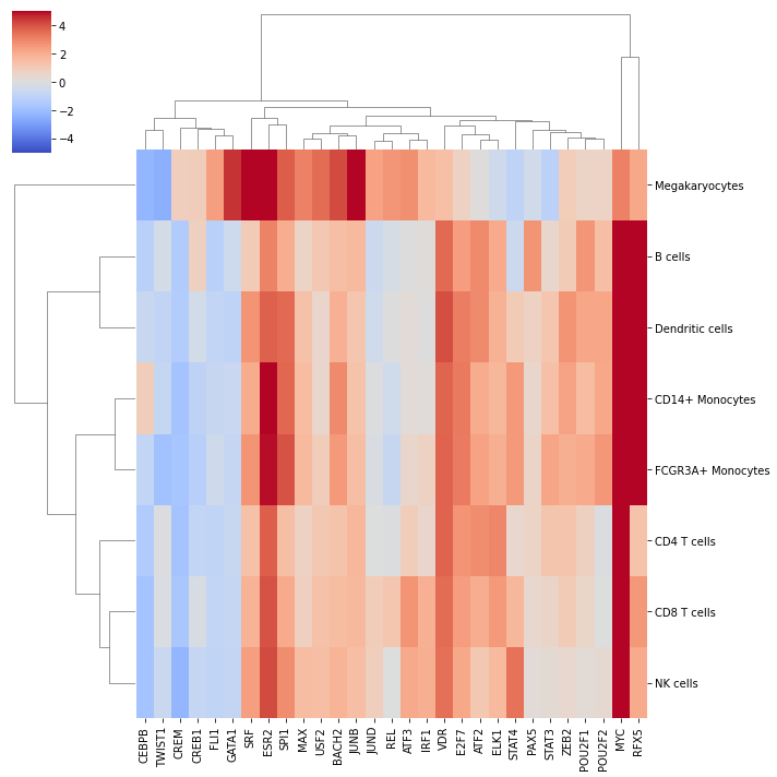
Here we can observe other known marker TFs appering, GATA1 for megakaryocytes, RFX5 for the myeloid lineage and JUND for the lymphoid.