Pathway activity inference

scRNA-seq yield many molecular readouts that are hard to interpret by themselves. One way of summarizing this information is by infering pathway activities from prior knowledge.

In this notebook we showcase how to use decoupler for pathway activity inference with the 3k PBMCs 10X data-set. The data consists of 3k PBMCs from a Healthy Donor and is freely available from 10x Genomics here from this webpage

Note

This tutorial assumes that you already know the basics of decoupler. Else, check out the Usage tutorial first.

Loading packages

First, we need to load the relevant packages, scanpy to handle scRNA-seq data and decoupler to use statistical methods.

import scanpy as sc
import decoupler as dc

# Only needed for visualization:
import matplotlib.pyplot as plt
import seaborn as sns

Loading the data

We can download the data easily using scanpy:

adata = sc.datasets.pbmc3k_processed()
adata

AnnData object with n_obs × n_vars = 2638 × 1838
    obs: 'n_genes', 'percent_mito', 'n_counts', 'louvain'
    var: 'n_cells'
    uns: 'draw_graph', 'louvain', 'louvain_colors', 'neighbors', 'pca', 'rank_genes_groups'
    obsm: 'X_pca', 'X_tsne', 'X_umap', 'X_draw_graph_fr'
    varm: 'PCs'
    obsp: 'distances', 'connectivities'

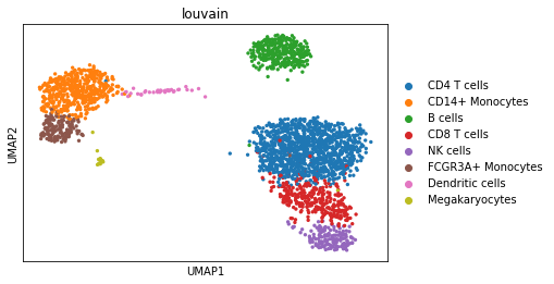
We can visualize the different cell types in it:

sc.pl.umap(adata, color='louvain')

PROGENy model

PROGENy is a comprehensive resource containing a curated collection of pathways and their target genes, with weights for each interaction. For this example we will use the human weights (mouse is also available) and we will use the top 500 responsive genes ranked by p-value. To access it we can use decoupler.

model = dc.get_progeny(organism='human', top=100)
model

	source	target	weight	p_value
0	Androgen	TMPRSS2	11.490631	0.000000e+00
1	Androgen	NKX3-1	10.622551	2.242078e-44
2	Androgen	MBOAT2	10.472733	4.624285e-44
3	Androgen	KLK2	10.176186	1.944414e-40
4	Androgen	SARG	11.386852	2.790209e-40
...	...	...	...	...
1395	p53	CCDC150	-3.174527	7.396252e-13
1396	p53	LCE1A	6.154823	8.475458e-13
1397	p53	TREM2	4.101937	9.739648e-13
1398	p53	GDF9	3.355741	1.087433e-12
1399	p53	NHLH2	2.201638	1.651582e-12

1399 rows × 4 columns

Activity inference with Multivariate Linear Model

To infer activities we will run the Multivariate Linear Model method (mlm), but we could do it with any of the other available methods in decoupler. It models the observed gene expression by using a regulatory adjacency matrix (target genes x pathways) as covariates of the linear model. The values of this matrix are the associated interaction weights. The obtained t-values of the fitted model are the activity scores.

To run decoupler methods, we need an input matrix (mat), an input prior knowledge network/resource (net), and the name of the columns of net that we want to use.

dc.run_mlm(mat=adata, net=model, source='source', target='target', weight='weight', verbose=True)

58 features of mat are empty in 2635 samples, they will be ignored.
Running mlm on mat with 2638 samples and 13656 targets for 14 sources.

100%|██████████████████████████████████████████████████████████████████████████████████████████████████████████████████████████████████████| 1/1 [00:01<00:00,  1.94s/it]

The obtained scores (t-values)(mlm_estimate) and p-values (mlm_pvals) are stored in the .obsm key:

adata.obsm['mlm_estimate']

	Androgen	EGFR	Estrogen	Hypoxia	JAK-STAT	MAPK	NFkB	PI3K	TGFb	TNFa	Trail	VEGF	WNT	p53
AAACATACAACCAC-1	-0.254317	1.089780	-0.285944	-0.028451	-1.106676	-1.430918	-0.082617	-0.799225	-1.149151	0.683357	-0.574796	0.116908	0.123379	0.050985
AAACATTGAGCTAC-1	0.049446	1.759345	-0.642154	0.473962	0.044179	-2.562641	0.499121	-0.047695	-1.256537	-0.668796	0.662174	0.320892	-0.886163	-1.080358
AAACATTGATCAGC-1	-1.303944	1.006542	-1.424544	0.786387	0.760430	-1.441959	-0.092619	-0.283998	-0.821725	0.893218	0.002368	0.186232	-0.380458	-0.004201
AAACCGTGCTTCCG-1	-1.112396	0.630100	-0.535417	0.392984	5.351217	-1.160324	-1.695362	-0.321097	-0.656579	1.709239	-0.192299	-0.466829	-0.293918	-1.363845
AAACCGTGTATGCG-1	-0.024953	-0.948639	0.111272	0.429596	1.997739	1.372292	-0.279557	0.023725	-0.366050	-0.005059	0.697554	-0.186563	-1.324360	-0.745233
...	...	...	...	...	...	...	...	...	...	...	...	...	...	...
TTTCGAACTCTCAT-1	-1.313557	1.648253	-0.521621	0.790064	5.908739	-1.281623	-2.046168	0.868645	-0.129498	2.279371	-0.395457	0.120466	0.379346	-0.726746
TTTCTACTGAGGCA-1	-0.089930	-0.266863	-0.336525	0.483492	1.307536	-0.548193	-0.635640	0.278944	-1.501156	0.174171	0.219865	0.288032	-0.357290	-0.364802
TTTCTACTTCCTCG-1	-0.384898	0.300295	-0.584879	-0.507010	0.398958	-0.775586	-1.212414	-1.737502	-0.691626	1.493439	1.031381	0.233926	-0.592165	-0.911064
TTTGCATGAGAGGC-1	-0.081229	1.168600	-0.053427	-0.944615	-1.009061	-1.175667	-0.632222	0.766005	-0.935478	0.303974	2.430962	-0.152354	0.621728	-0.182400
TTTGCATGCCTCAC-1	-0.215304	0.504166	0.697149	0.182862	1.069094	-0.979595	-0.787906	-1.315958	-0.760032	1.247450	0.310483	0.139131	0.036891	-1.155540

2638 rows × 14 columns

Visualization

To visualize the obtained scores, we can re-use many of scanpy’s plotting functions. First though, we need to extract the activities from the adata object.

acts = dc.get_acts(adata, obsm_key='mlm_estimate')
acts

AnnData object with n_obs × n_vars = 2638 × 14
    obs: 'n_genes', 'percent_mito', 'n_counts', 'louvain'
    uns: 'draw_graph', 'louvain', 'louvain_colors', 'neighbors', 'pca', 'rank_genes_groups'
    obsm: 'X_pca', 'X_tsne', 'X_umap', 'X_draw_graph_fr', 'mlm_estimate', 'mlm_pvals'

dc.get_acts returns a new AnnData object which holds the obtained activities in its .X attribute, allowing us to re-use many scanpy functions, for example:

sc.pl.umap(acts, color='Trail', vcenter=0, cmap='coolwarm')

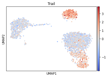
It seem that in B and NK cells, Trail is more active.

Exploration

With decoupler we can also see what is the mean activity per group:

mean_acts = dc.summarize_acts(acts, groupby='louvain', min_std=0)
mean_acts

	Androgen	EGFR	Estrogen	Hypoxia	JAK-STAT	MAPK	NFkB	PI3K	TGFb	TNFa	Trail	VEGF	WNT	p53
B cells	-0.468660	0.335794	-0.417370	-0.158317	0.814589	-0.857039	-0.588585	-0.209821	-0.882279	0.643021	1.154475	-0.204467	-0.220083	-0.571815
CD14+ Monocytes	-0.757344	1.043115	-0.491045	0.746968	2.380828	-1.356209	-0.985047	-0.224317	-0.775379	1.474249	-0.269548	-0.301558	0.006884	-0.576530
CD4 T cells	-0.739310	0.400723	-0.442679	0.255880	0.943968	-0.816171	-0.495911	-0.644359	-0.891962	0.913992	-0.273612	0.058542	-0.229659	-0.631909
CD8 T cells	-0.729621	0.446179	-0.409576	0.302857	1.101982	-0.856753	-0.754864	-0.347066	-0.993076	1.228680	0.293803	0.072465	-0.133162	-0.677359
Dendritic cells	-0.689440	1.091269	-0.639063	0.825579	3.071905	-1.574711	-0.519277	-0.528376	-0.770083	0.858204	-0.339843	-0.484117	0.182616	-0.613309
FCGR3A+ Monocytes	-0.869193	1.297832	-0.634357	0.868220	3.638588	-1.588427	-1.155033	-0.105399	-1.160496	1.756394	-0.231654	-0.363509	-0.361662	-0.638362
Megakaryocytes	-0.539666	2.370945	-0.379802	1.339065	0.074621	-2.264235	-0.628410	-0.999819	0.006513	0.659770	-0.047464	-0.015514	0.957362	-0.315593
NK cells	-0.695242	0.540878	-0.211991	0.382965	2.203062	-0.967779	-1.161683	-0.094474	-1.086600	1.237725	0.729644	0.240039	-0.098282	-0.713071

We can visualize which group is more active using seaborn:

sns.clustermap(mean_acts, xticklabels=mean_acts.columns, vmin=-2, vmax=2, cmap='coolwarm')
plt.show()

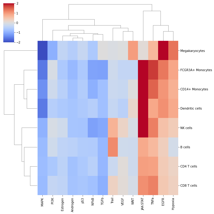
In this specific example, we can observe that WNT to be more active in Megakaryocytes, and that Trail is more active in B and NK cells.