Functional enrichment of biological terms
scRNA-seq yield many molecular readouts that are hard to interpret by themselves. One way of summarizing this information is by assigning them to biological terms from prior knowledge.
In this notebook we showcase how to use decoupler for functional enrichment with the 3k PBMCs 10X data-set. The data consists of 3k PBMCs from a Healthy Donor and is freely available from 10x Genomics here from this webpage
Note
This tutorial assumes that you already know the basics of decoupler. Else, check out the Usage tutorial first.
Loading packages
First, we need to load the relevant packages, scanpy to handle scRNA-seq data and decoupler to use statistical methods.
[1]:
import scanpy as sc
import decoupler as dc

# Only needed for visualization:
import matplotlib.pyplot as plt
import seaborn as sns
Loading the data
We can download the data easily using scanpy:
[2]:
adata = sc.datasets.pbmc3k_processed()
adata
[2]:
AnnData object with n_obs × n_vars = 2638 × 1838
    obs: 'n_genes', 'percent_mito', 'n_counts', 'louvain'
    var: 'n_cells'
    uns: 'draw_graph', 'louvain', 'louvain_colors', 'neighbors', 'pca', 'rank_genes_groups'
    obsm: 'X_pca', 'X_tsne', 'X_umap', 'X_draw_graph_fr'
    varm: 'PCs'
    obsp: 'distances', 'connectivities'
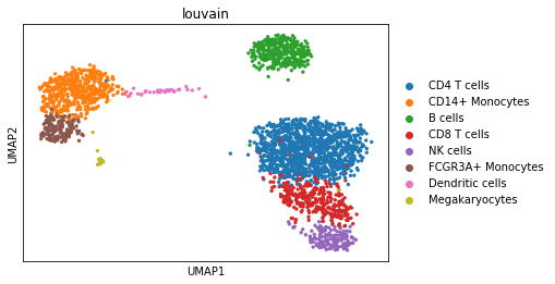
We can visualize the different cell types in it:
[3]:
sc.pl.umap(adata, color='louvain')
MSigDB gene sets
The Molecular Signatures Database (MSigDB) is a resource containing a collection of gene sets annotated to different biological processes.
[4]:
msigdb = dc.get_resource('MSigDB')
msigdb
[4]:
| genesymbol | collection | geneset | |
|---|---|---|---|
| 0 | MSC | oncogenic_signatures | PKCA_DN.V1_DN |
| 1 | MSC | mirna_targets | MIR12123 |
| 2 | MSC | chemical_and_genetic_perturbations | NIKOLSKY_BREAST_CANCER_8Q12_Q22_AMPLICON |
| 3 | MSC | immunologic_signatures | GSE32986_UNSTIM_VS_GMCSF_AND_CURDLAN_LOWDOSE_S... |
| 4 | MSC | chemical_and_genetic_perturbations | BENPORATH_PRC2_TARGETS |
| ... | ... | ... | ... |
| 2407729 | OR2W5P | immunologic_signatures | GSE22601_DOUBLE_NEGATIVE_VS_CD8_SINGLE_POSITIV... |
| 2407730 | OR2W5P | immunologic_signatures | KANNAN_BLOOD_2012_2013_TIV_AGE_65PLS_REVACCINA... |
| 2407731 | OR52L2P | immunologic_signatures | GSE22342_CD11C_HIGH_VS_LOW_DECIDUAL_MACROPHAGE... |
| 2407732 | CSNK2A3 | immunologic_signatures | OCONNOR_PBMC_MENVEO_ACWYVAX_AGE_30_70YO_7DY_AF... |
| 2407733 | AQP12B | immunologic_signatures | MATSUMIYA_PBMC_MODIFIED_VACCINIA_ANKARA_VACCIN... |
2407734 rows × 3 columns
As an example, we will use the hallmark gene sets, but we could have used any other such as KEGG or REACTOME.
Note
To see what other collections are available in MSigDB, type: msigdb['collection'].unique().
We can filter by for hallmark:
[5]:
# Filter by hallmark
msigdb = msigdb[msigdb['collection']=='hallmark']

# Remove duplicated entries
msigdb = msigdb[~msigdb.duplicated(['geneset', 'genesymbol'])]
msigdb
[5]:
| genesymbol | collection | geneset | |
|---|---|---|---|
| 11 | MSC | hallmark | HALLMARK_TNFA_SIGNALING_VIA_NFKB |
| 149 | ICOSLG | hallmark | HALLMARK_TNFA_SIGNALING_VIA_NFKB |
| 223 | ICOSLG | hallmark | HALLMARK_INFLAMMATORY_RESPONSE |
| 270 | ICOSLG | hallmark | HALLMARK_ALLOGRAFT_REJECTION |
| 398 | FOSL2 | hallmark | HALLMARK_HYPOXIA |
| ... | ... | ... | ... |
| 878342 | FOXO1 | hallmark | HALLMARK_PANCREAS_BETA_CELLS |
| 878418 | GCG | hallmark | HALLMARK_PANCREAS_BETA_CELLS |
| 878512 | PDX1 | hallmark | HALLMARK_PANCREAS_BETA_CELLS |
| 878605 | INS | hallmark | HALLMARK_PANCREAS_BETA_CELLS |
| 878785 | SRP9 | hallmark | HALLMARK_PANCREAS_BETA_CELLS |
7318 rows × 3 columns
For this example we will use the resource MSigDB, but we could have used any other such as GO. To see the list of available resources inside Omnipath, run dc.show_resources()
Enrichment with Over Representation Analysis
To test if a gene set is enriched in a given cell, we will run Over Representation Analysis (ora), also known as Fisher exact test, but we could do it with any of the other available methods in decoupler.
ora selects the top 5% expressed genes for each cell, and tests if a gene set is enriched in the top (or bottom) expressed collection.
To run decoupler methods, we need an input matrix (mat), an input prior knowledge network/resource (net), and the name of the columns of net that we want to use.
[6]:
dc.run_ora(mat=adata, net=msigdb, source='geneset', target='genesymbol', verbose=True)
1 features of mat are empty, they will be removed.
Running ora on mat with 2638 samples and 13713 targets for 50 sources.
100%|██████████████████████████████████████████████████████████████████████████████████████████████████████████████████████████████| 2638/2638 [00:02<00:00, 1088.99it/s]
The obtained scores (-log10(p-value))(ora_estimate) and p-values (ora_pvals) are stored in the .obsm key:
[7]:
adata.obsm['ora_estimate']
[7]:
| source | HALLMARK_ADIPOGENESIS | HALLMARK_ALLOGRAFT_REJECTION | HALLMARK_ANDROGEN_RESPONSE | HALLMARK_ANGIOGENESIS | HALLMARK_APICAL_JUNCTION | HALLMARK_APICAL_SURFACE | HALLMARK_APOPTOSIS | HALLMARK_BILE_ACID_METABOLISM | HALLMARK_CHOLESTEROL_HOMEOSTASIS | HALLMARK_COAGULATION | ... | HALLMARK_PROTEIN_SECRETION | HALLMARK_REACTIVE_OXYGEN_SPECIES_PATHWAY | HALLMARK_SPERMATOGENESIS | HALLMARK_TGF_BETA_SIGNALING | HALLMARK_TNFA_SIGNALING_VIA_NFKB | HALLMARK_UNFOLDED_PROTEIN_RESPONSE | HALLMARK_UV_RESPONSE_DN | HALLMARK_UV_RESPONSE_UP | HALLMARK_WNT_BETA_CATENIN_SIGNALING | HALLMARK_XENOBIOTIC_METABOLISM |
|---|---|---|---|---|---|---|---|---|---|---|---|---|---|---|---|---|---|---|---|---|---|
| AAACATACAACCAC-1 | 1.307006 | 10.029702 | 0.822139 | 0.389675 | 1.670031 | 0.650245 | 2.441094 | 0.337563 | 0.805206 | 0.032740 | ... | 0.733962 | 2.286568 | 0.354931 | 2.986336 | 8.220117 | 6.365243 | 0.586324 | 1.983873 | 0.164805 | 0.080157 |
| AAACATTGAGCTAC-1 | 1.307006 | 14.824230 | 2.152116 | 0.389675 | 2.104104 | -0.000000 | 0.442704 | 0.337563 | 0.457516 | 0.321093 | ... | 2.496213 | 1.659624 | 1.015676 | 1.659624 | 3.027820 | 2.547763 | 0.346751 | 0.871448 | 0.503794 | 0.080157 |
| AAACATTGATCAGC-1 | 3.893118 | 7.893567 | 3.312021 | 0.389675 | 3.095283 | 0.650245 | 5.115631 | 0.976973 | 0.805206 | 0.321093 | ... | 1.087271 | 3.752012 | 0.037885 | 1.114303 | 7.549513 | 2.048977 | 0.888675 | 4.038435 | 0.164805 | 1.087420 |
| AAACCGTGCTTCCG-1 | 5.591584 | 7.893567 | 2.152116 | 1.036748 | 1.670031 | -0.000000 | 2.911700 | 0.143019 | 1.747025 | 0.591452 | ... | 1.501986 | 3.752012 | 0.354931 | 1.659624 | 5.669689 | 4.950302 | 0.346751 | 1.567924 | 0.164805 | 1.087420 |
| AAACCGTGTATGCG-1 | 0.999733 | 10.029702 | 2.707608 | 1.871866 | 1.670031 | 1.948869 | 0.666121 | 0.337563 | 0.805206 | 0.591452 | ... | 1.973108 | 1.659624 | 0.151790 | 1.114303 | 1.785917 | 1.596582 | 0.586324 | 0.375221 | 0.164805 | 0.179270 |
| ... | ... | ... | ... | ... | ... | ... | ... | ... | ... | ... | ... | ... | ... | ... | ... | ... | ... | ... | ... | ... | ... |
| TTTCGAACTCTCAT-1 | 3.382339 | 9.297059 | 1.204403 | 1.036748 | 2.580035 | 0.224257 | 10.804691 | 0.143019 | 2.324194 | 1.359530 | ... | 3.683543 | 3.752012 | 0.151790 | 2.286568 | 5.669689 | 2.048977 | 0.586324 | 4.639190 | 0.164805 | 1.087420 |
| TTTCTACTGAGGCA-1 | 6.851412 | 4.777953 | 6.964458 | 1.036748 | 1.670031 | 0.650245 | 2.006125 | 0.035215 | 0.457516 | 1.359530 | ... | 3.683543 | 1.659624 | 0.151790 | 2.286568 | 2.168128 | 8.718220 | 0.172992 | 2.441252 | 0.164805 | 0.080157 |
| TTTCTACTTCCTCG-1 | 1.652714 | 7.224004 | 2.152116 | -0.000000 | 1.670031 | 1.235034 | 2.441094 | 0.337563 | 1.238111 | 0.134773 | ... | 1.087271 | 0.661862 | 0.151790 | 1.659624 | 8.911564 | 3.089847 | 0.064563 | 4.639190 | -0.000000 | 0.329247 |
| TTTGCATGAGAGGC-1 | 2.034899 | 5.352930 | 1.204403 | 1.036748 | 0.939005 | 1.235034 | 0.267770 | 0.617706 | 0.805206 | 0.134773 | ... | 0.733962 | 2.286568 | 0.151790 | 0.661862 | 3.502378 | 5.641478 | 0.346751 | 2.441252 | 0.164805 | 0.329247 |
| TTTGCATGCCTCAC-1 | 1.307006 | 10.029702 | 0.508632 | 0.389675 | 1.670031 | 0.650245 | 3.416073 | 0.976973 | 0.457516 | 0.134773 | ... | 0.232568 | 2.286568 | 0.037885 | 1.659624 | 3.502378 | 4.950302 | 0.888675 | 4.038435 | 0.164805 | 0.080157 |
2638 rows × 50 columns
Visualization
To visualize the obtianed scores, we can re-use many of scanpy’s plotting functions. First though, we need to extract them from the adata object.
[8]:
acts = dc.get_acts(adata, obsm_key='ora_estimate')
acts
[8]:
AnnData object with n_obs × n_vars = 2638 × 50
    obs: 'n_genes', 'percent_mito', 'n_counts', 'louvain'
    uns: 'draw_graph', 'louvain', 'louvain_colors', 'neighbors', 'pca', 'rank_genes_groups'
    obsm: 'X_pca', 'X_tsne', 'X_umap', 'X_draw_graph_fr', 'ora_estimate', 'ora_pvals'
dc.get_acts returns a new AnnData object which holds the obtained activities in its .X attribute, allowing us to re-use many scanpy functions, for example:
[9]:
sc.pl.umap(acts, color='HALLMARK_COAGULATION')
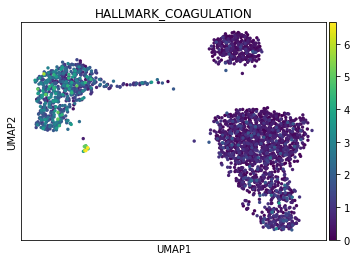
The cells highlighted seem to be enriched by coagulation.
Exploration
With decoupler we can also see what is the mean enrichment per group:
[10]:
mean_enr = dc.summarize_acts(acts, groupby='louvain', min_std=1)
mean_enr
[10]:
| HALLMARK_ALLOGRAFT_REJECTION | HALLMARK_APOPTOSIS | HALLMARK_COAGULATION | HALLMARK_COMPLEMENT | HALLMARK_HYPOXIA | HALLMARK_INTERFERON_ALPHA_RESPONSE | HALLMARK_INTERFERON_GAMMA_RESPONSE | HALLMARK_MYC_TARGETS_V1 | HALLMARK_OXIDATIVE_PHOSPHORYLATION | HALLMARK_TNFA_SIGNALING_VIA_NFKB | |
|---|---|---|---|---|---|---|---|---|---|---|
| B cells | 8.354994 | 1.917664 | 0.290295 | 1.229005 | 4.229028 | 5.219356 | 7.148639 | 18.921244 | 7.434455 | 3.780326 |
| CD14+ Monocytes | 7.548974 | 4.732542 | 1.753238 | 6.105103 | 5.718626 | 6.597623 | 9.203345 | 15.001544 | 10.768515 | 6.447618 |
| CD4 T cells | 7.367119 | 2.989820 | 0.404844 | 1.667583 | 5.704934 | 5.119762 | 5.761981 | 20.898235 | 8.849491 | 4.792259 |
| CD8 T cells | 10.050341 | 2.916126 | 0.551194 | 3.018337 | 5.510883 | 5.461279 | 7.221680 | 19.887226 | 8.511161 | 4.978559 |
| Dendritic cells | 11.001875 | 4.818395 | 1.361634 | 4.210152 | 6.341395 | 8.200227 | 11.063760 | 25.464518 | 15.929270 | 6.571718 |
| FCGR3A+ Monocytes | 9.142790 | 4.914899 | 2.015463 | 7.896366 | 6.478059 | 9.304629 | 11.687559 | 17.928917 | 13.115271 | 5.791608 |
| Megakaryocytes | 4.484497 | 3.401895 | 4.256961 | 3.466092 | 2.935619 | 1.846708 | 1.656383 | 5.570364 | 5.332106 | 3.127663 |
| NK cells | 10.658255 | 2.931217 | 0.644769 | 3.999646 | 5.708977 | 7.291569 | 9.032887 | 18.066849 | 8.723539 | 3.751579 |
We can visualize which group is more enriched using seaborn:
[11]:
sns.clustermap(mean_enr, xticklabels=mean_enr.columns, vmax=20, cmap='viridis')
plt.show()
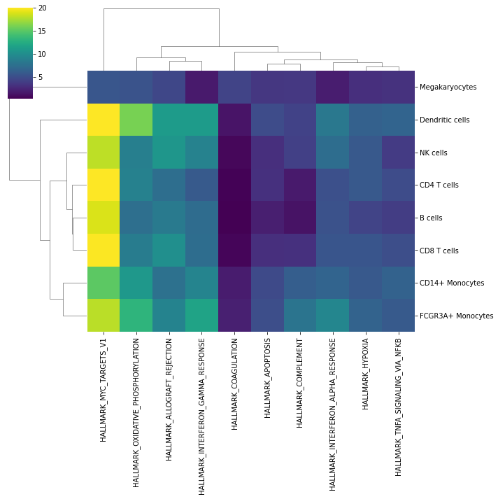
In this specific example, we can observe that most cell types are enriched by targets of MYC, a global regulator of the immune system, and megakaryocytes are enriched by coagulation genes.
Note
If your data consist of different conditions with enough samples, we recommend to work with pseudo-bulk profiles instead. Check this vignette for more informatin.