Spatial functional analysis

Spatial transcriptomics technologies yield many molecular readouts that are hard to interpret by themselves. One way of summarizing this information is by inferring biological activities from prior knowledge.

In this notebook we showcase how to use decoupler for transcription factor and pathway activity inference from a human data-set. The data consists of a 10X Genomics Visium slide of a human lymph node and it is available at their website.

Note

This tutorial assumes that you already know the basics of decoupler. Else, check out the Usage tutorial first.

Loading packages

First, we need to load the relevant packages, scanpy to handle RNA-seq data and decoupler to use statistical methods.

[1]:

import scanpy as sc
import decoupler as dc

# Only needed for processing and plotting
import numpy as np
import pandas as pd
import matplotlib.pyplot as plt
import seaborn as sns

Loading the data

We can download the data easily using scanpy:

[2]:

adata = sc.datasets.visium_sge(sample_id="V1_Human_Lymph_Node")
adata.var_names_make_unique()
adata

Variable names are not unique. To make them unique, call `.var_names_make_unique`.
Variable names are not unique. To make them unique, call `.var_names_make_unique`.

[2]:

AnnData object with n_obs × n_vars = 4035 × 36601
    obs: 'in_tissue', 'array_row', 'array_col'
    var: 'gene_ids', 'feature_types', 'genome'
    uns: 'spatial'
    obsm: 'spatial'

QC, projection and clustering

Here we follow the standard pre-processing steps as described in the scanpy vignette. These steps carry out the selection and filtration of spots based on quality control metrics, the data normalization and scaling, and the detection of highly variable features.

Note

This is just an example, these steps should change depending on the data.

[3]:

# Basic filtering
sc.pp.filter_cells(adata, min_genes=200)
sc.pp.filter_genes(adata, min_cells=10)

# Annotate the group of mitochondrial genes as 'mt'
adata.var['mt'] = adata.var_names.str.startswith('MT-')
sc.pp.calculate_qc_metrics(adata, qc_vars=['mt'], percent_top=None, log1p=False, inplace=True)

# Filter cells following standard QC criteria.
adata = adata[adata.obs.pct_counts_mt < 20, :]

# Normalize the data
sc.pp.normalize_total(adata, target_sum=1e4)
sc.pp.log1p(adata)

# Identify highly variable genes
sc.pp.highly_variable_genes(adata)

# Filter higly variable genes
adata.raw = adata
adata = adata[:, adata.var.highly_variable]

# Scale the data
sc.pp.scale(adata, max_value=10)

/home/badi/miniconda3/envs/decoupler/lib/python3.8/site-packages/scanpy/preprocessing/_normalization.py:155: UserWarning: Revieved a view of an AnnData. Making a copy.
  view_to_actual(adata)
/home/badi/miniconda3/envs/decoupler/lib/python3.8/site-packages/scanpy/preprocessing/_simple.py:843: UserWarning: Revieved a view of an AnnData. Making a copy.
  view_to_actual(adata)

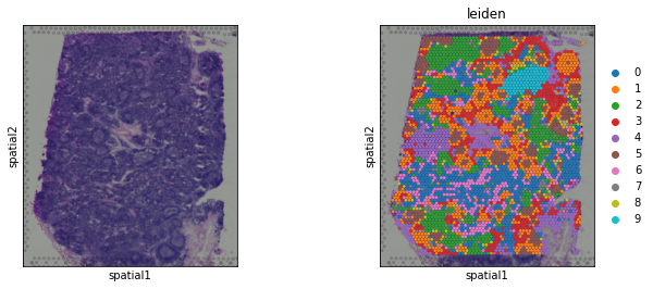
Then we group spots based on the similarity of their transcription profiles. We can visualize the obtianed clusters on a UMAP or directly at the tissue:

[4]:

# Generate PCA features
sc.tl.pca(adata, svd_solver='arpack')

# Compute distances in the PCA space, and find spot neighbors
sc.pp.neighbors(adata)

# Run leiden clustering algorithm
sc.tl.leiden(adata)

# Visualize
sc.pl.spatial(adata, color=[None, 'leiden'], size=1.5, wspace=0)

/home/badi/miniconda3/envs/decoupler/lib/python3.8/site-packages/anndata/_core/anndata.py:1220: FutureWarning: The `inplace` parameter in pandas.Categorical.reorder_categories is deprecated and will be removed in a future version. Reordering categories will always return a new Categorical object.
  c.reorder_categories(natsorted(c.categories), inplace=True)
... storing 'feature_types' as categorical
/home/badi/miniconda3/envs/decoupler/lib/python3.8/site-packages/anndata/_core/anndata.py:1220: FutureWarning: The `inplace` parameter in pandas.Categorical.reorder_categories is deprecated and will be removed in a future version. Reordering categories will always return a new Categorical object.
  c.reorder_categories(natsorted(c.categories), inplace=True)
... storing 'genome' as categorical

Transcription factor activity inference

The first functional analysis we can perform is to infer transcription factor (TF) activities from our transcriptomics data. We will need a gene regulatory network (GRN) and a statistical method.

DoRothEA network

DoRothEA is a comprehensive resource containing a curated collection of TFs and their transcriptional targets. Since these regulons were gathered from different types of evidence, interactions in DoRothEA are classified in different confidence levels, ranging from A (highest confidence) to D (lowest confidence). Moreover, each interaction is weighted by its confidence level and the sign of its mode of regulation (activation or inhibition).

For this example we will use the human version (other organisms are available) and we will use the confidence levels ABC. To access it we can use decoupler.

Note

In this tutorial we use the network DoRothEA, but we could use any other GRN coming from an inference method such as CellOracle, pySCENIC or SCENIC+.

[5]:

net = dc.get_dorothea(organism='human', levels=['A','B','C'])
net

[5]:

	source	confidence	target	weight
0	ETS1	A	IL12B	1.000000
1	RELA	A	IL6	1.000000
2	MITF	A	BCL2A1	-1.000000
3	E2F1	A	TRERF1	1.000000
4	MITF	A	BCL2	1.000000
...	...	...	...	...
32272	IKZF1	C	PTK2B	0.333333
32273	IKZF1	C	PRKCB	0.333333
32274	IKZF1	C	PREX1	0.333333
32275	IRF4	C	SLAMF7	0.333333
32276	ZNF83	C	ZNF331	0.333333

32277 rows × 4 columns

Activity inference with Multivariate Linear Model

To infer activities we will run the Multivariate Linear Model method (mlm). It models the observed gene expression by using a regulatory adjacency matrix (target genes x TFs) as covariates of a linear model. The values of this matrix are the associated interaction weights. The obtained t-values of the fitted model are the activity scores.

To run decoupler methods, we need an input matrix (mat), an input prior knowledge network/resource (net), and the name of the columns of net that we want to use.

[6]:

dc.run_mlm(mat=adata, net=net, source='source', target='target', weight='weight', verbose=True)

Running mlm on mat with 4032 samples and 19813 targets for 294 sources.

100%|██████████████████████████████████████████████████████████████████████████████████████████████████████████████████████████████████████| 1/1 [00:06<00:00,  6.84s/it]

The obtained scores (t-values)(mlm_estimate) and p-values (mlm_pvals) are stored in the .obsm key:

[7]:

adata.obsm['mlm_estimate']

[7]:

	AHR	AR	ARID2	ARID3A	ARNT	ARNTL	ASCL1	ATF1	ATF2	ATF3	...	ZNF217	ZNF24	ZNF263	ZNF274	ZNF384	ZNF584	ZNF592	ZNF639	ZNF644	ZNF740
AAACAAGTATCTCCCA-1	0.531388	4.314746	2.580497	-2.264766	-0.211907	0.031246	-0.705776	-0.118562	0.799197	-0.045215	...	0.618186	-0.924915	-1.565854	-0.710968	1.119455	0.527442	0.561804	3.302261	-0.169674	1.063122
AAACAATCTACTAGCA-1	-0.684831	3.082588	2.525492	-0.760523	-0.134987	-1.309098	-0.090339	-0.262004	1.189955	-0.133106	...	0.001439	-1.933857	-1.526967	-0.431441	0.914302	0.337622	1.228477	3.548201	-0.341155	0.854290
AAACACCAATAACTGC-1	-0.966583	3.456383	0.965503	-2.124058	-0.092816	-1.105180	-0.122935	1.216181	1.331234	0.694221	...	1.274752	-1.129040	-1.979256	0.094362	1.624496	0.581281	-0.018216	2.823706	-0.299057	0.781646
AAACAGAGCGACTCCT-1	0.084335	3.552887	2.330085	-1.771000	-0.805615	-0.930001	-0.450489	0.392044	1.208560	-0.174565	...	0.172208	-1.423535	-1.436785	-1.608596	1.548968	0.492690	0.748371	2.668740	1.290589	0.898669
AAACAGCTTTCAGAAG-1	-0.113021	3.062887	1.692873	-1.376210	-0.237199	-1.540030	0.218669	0.059750	1.091377	-0.090121	...	0.990816	-1.068140	-1.429415	-0.121686	0.748879	0.354986	0.187215	2.666389	0.885567	0.440206
...	...	...	...	...	...	...	...	...	...	...	...	...	...	...	...	...	...	...	...	...	...
TTGTTTCACATCCAGG-1	-0.890853	3.760496	1.341087	-2.143296	0.199219	-1.063316	0.574174	-0.232284	-0.531052	-0.697277	...	2.323004	-1.538032	-2.160935	-0.829605	0.601897	-0.741982	0.184341	2.963787	-0.056685	0.354788
TTGTTTCATTAGTCTA-1	1.157550	3.614088	0.934339	-1.603928	-1.034015	-1.440529	-0.260510	-0.934655	0.368782	0.272667	...	1.935458	-1.350134	-1.803886	-1.309194	0.239783	0.030232	-0.161986	3.265780	0.185732	2.117301
TTGTTTCCATACAACT-1	-1.258395	2.891093	3.206188	-1.074143	-0.382113	-0.945535	-0.151498	1.225757	1.193222	-0.135125	...	1.379948	-0.543945	-1.674882	-0.879069	1.404226	0.835917	-0.477097	2.610413	-0.327709	1.427865
TTGTTTGTATTACACG-1	-0.739230	2.823546	3.534382	-1.066094	0.324376	-1.311501	-1.026220	0.729384	1.583481	0.750026	...	0.692039	-1.517446	-1.793239	-0.583169	1.176431	0.302630	-0.199994	2.923765	-1.083028	0.244638
TTGTTTGTGTAAATTC-1	0.159324	3.061946	2.349993	-0.897393	0.464201	-1.336176	-0.436003	-0.506391	-0.004222	0.715258	...	0.998253	-1.181231	-0.979263	-1.144093	1.208452	0.733775	0.272451	3.959256	1.771204	1.412840

4032 rows × 294 columns

Note: Each run of run_mlm overwrites what is inside of mlm_estimate and mlm_pvals. if you want to run mlm with other resources and still keep the activities inside the same AnnData object, you can store the results in any other key in .obsm with different names, for example:

[8]:

adata.obsm['dorothea_mlm_estimate'] = adata.obsm['mlm_estimate'].copy()
adata.obsm['dorothea_mlm_pvals'] = adata.obsm['mlm_pvals'].copy()
adata

[8]:

AnnData object with n_obs × n_vars = 4032 × 2491
    obs: 'in_tissue', 'array_row', 'array_col', 'n_genes', 'n_genes_by_counts', 'total_counts', 'total_counts_mt', 'pct_counts_mt', 'leiden'
    var: 'gene_ids', 'feature_types', 'genome', 'n_cells', 'mt', 'n_cells_by_counts', 'mean_counts', 'pct_dropout_by_counts', 'total_counts', 'highly_variable', 'means', 'dispersions', 'dispersions_norm', 'mean', 'std'
    uns: 'spatial', 'log1p', 'hvg', 'pca', 'neighbors', 'leiden', 'leiden_colors'
    obsm: 'spatial', 'X_pca', 'mlm_estimate', 'mlm_pvals', 'dorothea_mlm_estimate', 'dorothea_mlm_pvals'
    varm: 'PCs'
    obsp: 'distances', 'connectivities'

Visualization

To visualize the obtained scores, we can re-use many of scanpy’s plotting functions. First though, we need to extract them from the adata object.

[9]:

acts = dc.get_acts(adata, obsm_key='dorothea_mlm_estimate')
acts

[9]:

AnnData object with n_obs × n_vars = 4032 × 294
    obs: 'in_tissue', 'array_row', 'array_col', 'n_genes', 'n_genes_by_counts', 'total_counts', 'total_counts_mt', 'pct_counts_mt', 'leiden'
    uns: 'spatial', 'log1p', 'hvg', 'pca', 'neighbors', 'leiden', 'leiden_colors'
    obsm: 'spatial', 'X_pca', 'mlm_estimate', 'mlm_pvals', 'dorothea_mlm_estimate', 'dorothea_mlm_pvals'

dc.get_acts returns a new AnnData object which holds the obtained activities in its .X attribute, allowing us to re-use many scanpy functions, for example:

[10]:

sc.pl.spatial(acts, color=['leiden', 'PAX5'], cmap='coolwarm', size=1.5, wspace=0)

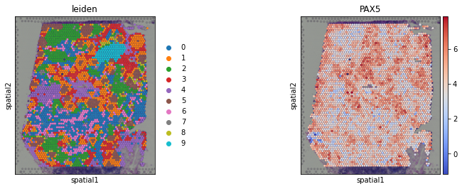
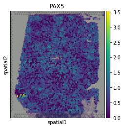
Here we observe the activity infered for PAX5 across spots. Interestingly, PAX5 is a known TF crucial for B cell identity and function. The inference of activities from “foot-prints” of target genes is more informative than just looking at the molecular readouts of a given TF, as an example here is the gene expression of PAX5, which is not very informative by itself:

[11]:

sc.pl.spatial(adata, color='PAX5', size=1.5)

Exploration

With decoupler we can also see what is the mean activity per group (to show more TFs, increase the min_std parameter):

[12]:

mean_acts = dc.summarize_acts(acts, groupby='leiden', min_std=0.4)
mean_acts

[12]:

	ATF6	E2F4	ERG	ETS1	IRF1	IRF9	JUNB	MYC	PAX5	RBPJ	RFX5	STAT1	STAT2	STAT3	TBX21	TFDP1
0	5.425647	5.950534	0.976629	7.022013	-0.296379	0.364462	1.528090	13.706879	3.980209	-0.702463	11.314269	1.457677	3.198416	2.211520	1.840758	1.651450
1	3.962387	6.329461	0.899010	7.067654	-0.045027	0.298553	2.174330	14.132327	5.419888	0.276466	12.545614	1.347172	3.390375	1.564702	1.688480	1.655355
2	4.308863	6.204994	0.908421	7.663957	-0.114513	0.257776	1.688271	14.019668	3.838306	-0.979750	10.227130	1.548294	3.774739	1.867868	2.608472	1.564099
3	4.677002	6.115650	1.481284	7.245724	-0.132964	0.336158	1.832213	14.238405	4.562850	-0.398871	12.552104	1.873078	3.420067	2.550702	1.399548	1.762380
4	4.512222	5.423492	1.353292	6.270385	-0.105885	0.345371	1.903540	13.461339	4.112409	-0.179700	11.339410	1.291094	2.708822	2.374198	1.275249	1.746006
5	3.962252	9.133594	0.696790	6.748394	-0.343900	0.270207	2.835591	14.928737	5.408315	0.556190	12.102087	0.981099	2.347938	1.259365	1.193647	4.038791
6	5.333444	5.908932	1.525536	7.519007	-0.266074	0.298177	1.360018	14.022554	4.233101	-0.598897	12.145805	1.924856	3.262287	2.700020	1.615572	1.588291
7	4.924606	6.188310	1.961460	7.522125	-0.171967	0.355779	1.561548	14.214684	3.937887	-0.789719	11.407527	1.688864	3.329131	2.477357	1.921157	1.785569
8	4.742176	7.305005	0.868916	7.338912	-0.117163	0.395704	1.915956	14.851122	4.743230	-0.567329	11.423132	1.358365	3.459237	1.808232	1.838801	2.466387
9	4.523947	6.937476	0.825905	7.283448	1.095696	1.769770	1.874522	14.956728	4.442098	-0.750603	10.470515	2.704625	10.020187	1.340084	2.119819	2.382874

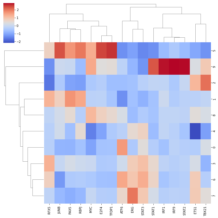
We can visualize which TF is more active across clusters using seaborn:

[13]:

sns.clustermap(mean_acts, xticklabels=mean_acts.columns, cmap='coolwarm', z_score=1)
plt.show()

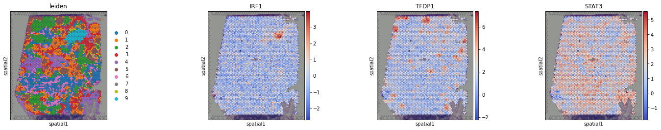
We can visualize again on the tissue some marker TFs:

[14]:

sc.pl.spatial(acts, color=['leiden', 'IRF1', 'TFDP1', 'STAT3'], cmap='coolwarm', size=1.5, wspace=0)

Pathway activity inference

We can also infer pathway activities from our transcriptomics data.

PROGENy model

PROGENy is a comprehensive resource containing a curated collection of pathways and their target genes, with weights for each interaction. For this example we will use the human weights (other organisms are available) and we will use the top 100 responsive genes ranked by p-value. Here is a brief description of each pathway:

Androgen: involved in the growth and development of the male reproductive organs.
EGFR: regulates growth, survival, migration, apoptosis, proliferation, and differentiation in mammalian cells
Estrogen: promotes the growth and development of the female reproductive organs.
Hypoxia: promotes angiogenesis and metabolic reprogramming when O2 levels are low.
JAK-STAT: involved in immunity, cell division, cell death, and tumor formation.
MAPK: integrates external signals and promotes cell growth and proliferation.
NFkB: regulates immune response, cytokine production and cell survival.
p53: regulates cell cycle, apoptosis, DNA repair and tumor suppression.
PI3K: promotes growth and proliferation.
TGFb: involved in development, homeostasis, and repair of most tissues.
TNFa: mediates haematopoiesis, immune surveillance, tumour regression and protection from infection.
Trail: induces apoptosis.
VEGF: mediates angiogenesis, vascular permeability, and cell migration.
WNT: regulates organ morphogenesis during development and tissue repair.

To access it we can use decoupler.

[15]:

model = dc.get_progeny(organism='human', top=100)
model

[15]:

	source	target	weight	p_value
0	Androgen	TMPRSS2	11.490631	0.000000e+00
1	Androgen	NKX3-1	10.622551	2.242078e-44
2	Androgen	MBOAT2	10.472733	4.624285e-44
3	Androgen	KLK2	10.176186	1.944414e-40
4	Androgen	SARG	11.386852	2.790209e-40
...	...	...	...	...
1395	p53	CCDC150	-3.174527	7.396252e-13
1396	p53	LCE1A	6.154823	8.475458e-13
1397	p53	TREM2	4.101937	9.739648e-13
1398	p53	GDF9	3.355741	1.087433e-12
1399	p53	NHLH2	2.201638	1.651582e-12

1400 rows × 4 columns

Activity inference with Multivariate Linear Model

Like in the previous section, we will use mlm to infer activities:

[16]:

dc.run_mlm(mat=adata, net=model, source='source', target='target', weight='weight', verbose=True)

# Store them in a different key
adata.obsm['progeny_mlm_estimate'] = adata.obsm['mlm_estimate'].copy()
adata.obsm['progeny_mlm_pvals'] = adata.obsm['mlm_pvals'].copy()

Running mlm on mat with 4032 samples and 19813 targets for 14 sources.

100%|██████████████████████████████████████████████████████████████████████████████████████████████████████████████████████████████████████| 1/1 [00:04<00:00,  4.79s/it]

The obtained scores (t-values)(mlm_estimate) and p-values (mlm_pvals) are stored in the .obsm key:

[17]:

adata.obsm['progeny_mlm_estimate']

[17]:

	Androgen	EGFR	Estrogen	Hypoxia	JAK-STAT	MAPK	NFkB	PI3K	TGFb	TNFa	Trail	VEGF	WNT	p53
AAACAAGTATCTCCCA-1	-0.188486	1.208809	0.845334	2.824020	2.956565	0.844544	-1.375955	-1.658008	-0.506245	3.400028	0.948775	0.354302	-0.394136	-0.592207
AAACAATCTACTAGCA-1	-0.296953	-0.593280	-0.558594	1.577488	3.994631	-0.434184	-0.145056	-2.026974	-1.356935	2.522995	0.198127	0.449313	-0.742038	0.015973
AAACACCAATAACTGC-1	-0.438746	0.179741	0.412451	1.812180	4.110078	0.803520	-1.396133	-2.972383	-1.486423	4.421825	0.567402	0.804890	-0.735639	0.174948
AAACAGAGCGACTCCT-1	0.007000	0.652227	-0.821658	2.101911	22.972557	-0.683112	-1.704974	-1.953475	-1.653204	3.975250	1.694650	0.755143	-0.501892	0.129601
AAACAGCTTTCAGAAG-1	-0.482217	0.393672	-0.576826	1.959044	4.177846	-0.527857	-0.996393	-3.752962	-1.633997	2.832229	0.967923	-0.093649	-0.575737	0.212081
...	...	...	...	...	...	...	...	...	...	...	...	...	...	...
TTGTTTCACATCCAGG-1	-0.292770	1.405961	0.330157	1.788581	4.066021	-0.854148	-1.628868	-2.403106	-1.488374	3.821350	0.888249	0.231786	-0.673330	-0.536630
TTGTTTCATTAGTCTA-1	0.216849	0.954299	-0.934332	2.779557	3.680631	0.638986	-0.052738	-1.530679	-1.766615	3.159299	-0.192867	0.422701	-0.358662	0.280121
TTGTTTCCATACAACT-1	-0.351691	0.822820	0.292143	1.386598	3.325152	0.149769	-0.320018	-2.387814	-0.621196	3.825063	0.242561	-0.025989	0.193019	0.199643
TTGTTTGTATTACACG-1	-1.506403	0.693628	-0.210152	2.470843	4.737563	-0.181501	-0.572574	-1.724866	-0.646039	2.713047	-0.016597	0.299411	-0.704308	-0.432493
TTGTTTGTGTAAATTC-1	-0.116604	0.914778	-0.572922	1.167968	4.379010	-1.397615	-0.151022	-2.901103	-2.101318	1.985720	0.722871	0.648947	-1.590521	0.610262

4032 rows × 14 columns

Visualization

Like in the previous section, we will extract the activities from the adata object.

[18]:

acts = dc.get_acts(adata, obsm_key='progeny_mlm_estimate')
acts

[18]:

AnnData object with n_obs × n_vars = 4032 × 14
    obs: 'in_tissue', 'array_row', 'array_col', 'n_genes', 'n_genes_by_counts', 'total_counts', 'total_counts_mt', 'pct_counts_mt', 'leiden'
    uns: 'spatial', 'log1p', 'hvg', 'pca', 'neighbors', 'leiden', 'leiden_colors'
    obsm: 'spatial', 'X_pca', 'mlm_estimate', 'mlm_pvals', 'dorothea_mlm_estimate', 'dorothea_mlm_pvals', 'progeny_mlm_estimate', 'progeny_mlm_pvals'

Once extracted we can visualize them:

[19]:

sc.pl.spatial(acts, color='Trail', cmap='coolwarm', size=1.5)

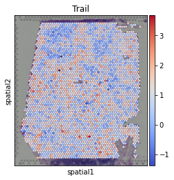
Here we show the activity of the pathway Trail, which is associated with apoptosis.

Exploration

Let us see the mean pathway activity per cluster:

[20]:

mean_acts = dc.summarize_acts(acts, groupby='leiden', min_std=0)
mean_acts

[20]:

	Androgen	EGFR	Estrogen	Hypoxia	JAK-STAT	MAPK	NFkB	PI3K	TGFb	TNFa	Trail	VEGF	WNT	p53
0	-0.235733	0.390685	0.057316	2.028656	3.310778	-0.082057	-0.693550	-2.151323	-1.103416	2.876699	0.877714	0.212958	-0.744617	0.018514
1	-0.361732	0.395693	-0.508569	1.789956	3.559256	-0.339410	-0.866924	-2.090730	-1.236661	2.921738	1.268237	0.484229	-0.683389	-0.038626
2	-0.376320	0.267465	-0.413390	2.016582	3.970872	-0.114459	-0.707642	-2.385279	-1.294334	3.097718	0.508334	0.561026	-0.735835	0.041692
3	-0.247242	0.840521	-0.134884	2.248527	3.830161	-0.104251	-0.472488	-2.093627	-0.693436	3.823169	1.041569	0.493589	-0.611709	0.063977
4	-0.262289	0.643110	0.029117	1.830205	3.153491	-0.335399	-0.823879	-1.951632	-0.444595	3.039439	1.043293	0.136829	-0.619363	-0.133458
5	0.055557	0.533585	-0.446169	1.856608	2.214398	-0.528827	-1.073485	-1.667952	-1.513876	2.833984	1.222594	0.461531	-0.993194	-0.156339
6	-0.157354	0.582798	0.130340	2.260429	3.516362	0.081085	-0.560231	-2.286241	-0.858187	3.446463	0.952809	0.367802	-0.633847	0.089529
7	-0.203110	0.504909	0.016051	2.047894	3.947978	-0.105809	-0.891699	-2.283474	-0.394168	3.202955	0.720393	0.497918	-0.659265	0.014837
8	-0.186089	0.454411	-0.238047	2.045116	3.660860	-0.251945	-0.904483	-2.138275	-1.225798	2.962659	0.756347	0.422399	-0.794784	-0.045474
9	-0.292553	0.451394	-0.383922	2.077637	14.496776	-0.136514	-1.136826	-2.143701	-1.429141	3.352161	0.555814	0.549724	-0.665753	-0.115536

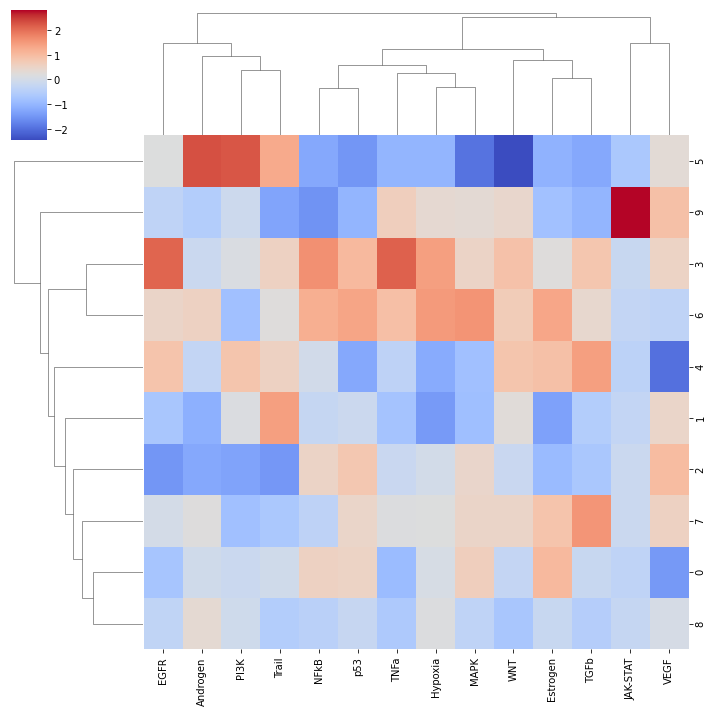
And visualize them:

[21]:

sns.clustermap(mean_acts, xticklabels=mean_acts.columns, cmap='coolwarm', z_score=1)
plt.show()

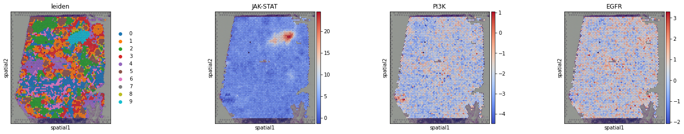
We can visualize again on the tissue some cluster-specific pathways:

[22]:

sc.pl.spatial(acts, color=['leiden', 'JAK-STAT', 'PI3K', 'EGFR'], cmap='coolwarm', size=1.5, wspace=0)

Functional enrichment of biological terms

Finally, we can also infer activities for general biological terms or processes.

MSigDB gene sets

The Molecular Signatures Database (MSigDB) is a resource containing a collection of gene sets annotated to different biological processes.

[23]:

msigdb = dc.get_resource('MSigDB')
msigdb

[23]:

	genesymbol	collection	geneset
0	MSC	oncogenic_signatures	PKCA_DN.V1_DN
1	MSC	mirna_targets	MIR12123
2	MSC	chemical_and_genetic_perturbations	NIKOLSKY_BREAST_CANCER_8Q12_Q22_AMPLICON
3	MSC	immunologic_signatures	GSE32986_UNSTIM_VS_GMCSF_AND_CURDLAN_LOWDOSE_S...
4	MSC	chemical_and_genetic_perturbations	BENPORATH_PRC2_TARGETS
...	...	...	...
2407729	OR2W5P	immunologic_signatures	GSE22601_DOUBLE_NEGATIVE_VS_CD8_SINGLE_POSITIV...
2407730	OR2W5P	immunologic_signatures	KANNAN_BLOOD_2012_2013_TIV_AGE_65PLS_REVACCINA...
2407731	OR52L2P	immunologic_signatures	GSE22342_CD11C_HIGH_VS_LOW_DECIDUAL_MACROPHAGE...
2407732	CSNK2A3	immunologic_signatures	OCONNOR_PBMC_MENVEO_ACWYVAX_AGE_30_70YO_7DY_AF...
2407733	AQP12B	immunologic_signatures	MATSUMIYA_PBMC_MODIFIED_VACCINIA_ANKARA_VACCIN...

2407734 rows × 3 columns

As an example, we will use the hallmark gene sets, but we could have used any other.

Note

To see what other collections are available in MSigDB, type: msigdb['collection'].unique().

We can filter by for hallmark:

[24]:

# Filter by hallmark
msigdb = msigdb[msigdb['collection']=='hallmark']

# Remove duplicated entries
msigdb = msigdb[~msigdb.duplicated(['geneset', 'genesymbol'])]

# Rename
msigdb.loc[:, 'geneset'] = [name.split('HALLMARK_')[1] for name in msigdb['geneset']]

msigdb

[24]:

	genesymbol	collection	geneset
11	MSC	hallmark	TNFA_SIGNALING_VIA_NFKB
149	ICOSLG	hallmark	TNFA_SIGNALING_VIA_NFKB
223	ICOSLG	hallmark	INFLAMMATORY_RESPONSE
270	ICOSLG	hallmark	ALLOGRAFT_REJECTION
398	FOSL2	hallmark	HYPOXIA
...	...	...	...
878342	FOXO1	hallmark	PANCREAS_BETA_CELLS
878418	GCG	hallmark	PANCREAS_BETA_CELLS
878512	PDX1	hallmark	PANCREAS_BETA_CELLS
878605	INS	hallmark	PANCREAS_BETA_CELLS
878785	SRP9	hallmark	PANCREAS_BETA_CELLS

7318 rows × 3 columns

Activity inference with Multivariate Linear Model

Like in the previous section, we will use mlm to infer activities:

[25]:

dc.run_mlm(mat=adata, net=msigdb, source='geneset', target='genesymbol', weight=None, verbose=True)

# Store them in a different key
adata.obsm['msigdb_mlm_estimate'] = adata.obsm['mlm_estimate'].copy()
adata.obsm['msigdb_mlm_pvals'] = adata.obsm['mlm_pvals'].copy()

Running mlm on mat with 4032 samples and 19813 targets for 50 sources.

100%|██████████████████████████████████████████████████████████████████████████████████████████████████████████████████████████████████████| 1/1 [00:04<00:00,  4.03s/it]

The obtained scores (t-values)(mlm_estimate) and p-values (mlm_pvals) are stored in the .obsm key:

[26]:

adata.obsm['msigdb_mlm_estimate'].iloc[:, 0:5]

[26]:

	ADIPOGENESIS	ALLOGRAFT_REJECTION	ANDROGEN_RESPONSE	ANGIOGENESIS	APICAL_JUNCTION
AAACAAGTATCTCCCA-1	3.582305	11.334203	4.234747	0.137435	3.802077
AAACAATCTACTAGCA-1	2.671094	12.194424	2.753398	-0.224686	2.211782
AAACACCAATAACTGC-1	3.254313	11.859533	4.187515	-0.349350	3.922884
AAACAGAGCGACTCCT-1	1.460420	11.618388	4.099222	-0.313021	4.280679
AAACAGCTTTCAGAAG-1	1.603691	12.120145	2.952333	-0.271135	2.790807
...	...	...	...	...	...
TTGTTTCACATCCAGG-1	2.417024	9.619124	4.501319	0.699741	3.429903
TTGTTTCATTAGTCTA-1	3.775330	11.446894	4.151324	0.583313	5.161738
TTGTTTCCATACAACT-1	2.932805	12.189088	3.406567	-0.550669	4.736694
TTGTTTGTATTACACG-1	1.151807	10.742589	2.760084	-0.723917	3.925781
TTGTTTGTGTAAATTC-1	1.686387	11.515235	3.075319	-1.084208	3.733509

4032 rows × 5 columns

Visualization

Like in the previous sections, we will extract the activities from the adata object.

[27]:

acts = dc.get_acts(adata, obsm_key='msigdb_mlm_estimate')
acts

[27]:

AnnData object with n_obs × n_vars = 4032 × 50
    obs: 'in_tissue', 'array_row', 'array_col', 'n_genes', 'n_genes_by_counts', 'total_counts', 'total_counts_mt', 'pct_counts_mt', 'leiden'
    uns: 'spatial', 'log1p', 'hvg', 'pca', 'neighbors', 'leiden', 'leiden_colors'
    obsm: 'spatial', 'X_pca', 'mlm_estimate', 'mlm_pvals', 'dorothea_mlm_estimate', 'dorothea_mlm_pvals', 'progeny_mlm_estimate', 'progeny_mlm_pvals', 'msigdb_mlm_estimate', 'msigdb_mlm_pvals'

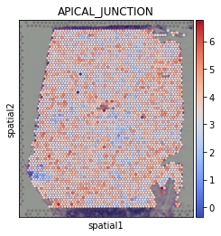
Once extracted we can visualize them:

[28]:

sc.pl.spatial(acts, color='APICAL_JUNCTION', cmap='coolwarm', size=1.5)

Exploration

Let us see the most variable terms:

[29]:

mean_acts = dc.summarize_acts(acts, groupby='leiden', min_std=0.35)
mean_acts

[29]:

	COAGULATION	DNA_REPAIR	E2F_TARGETS	EPITHELIAL_MESENCHYMAL_TRANSITION	G2M_CHECKPOINT	INTERFERON_ALPHA_RESPONSE	INTERFERON_GAMMA_RESPONSE	KRAS_SIGNALING_UP	MYC_TARGETS_V1	OXIDATIVE_PHOSPHORYLATION	TNFA_SIGNALING_VIA_NFKB	UNFOLDED_PROTEIN_RESPONSE
0	0.952400	3.288563	1.090645	1.618884	2.080138	3.904741	5.837221	1.469192	18.919279	10.948023	3.336524	6.792207
1	0.507895	3.667026	1.263194	0.769735	2.176249	4.147588	5.594840	1.383072	19.796711	11.067318	2.634282	5.720784
2	0.713078	3.559376	0.962561	1.215796	1.934632	4.388570	5.846885	1.429250	19.889725	11.445617	3.115541	6.276733
3	1.784987	3.652838	0.858465	2.945634	1.832419	4.097078	6.311147	2.180722	20.106998	11.705830	4.497266	6.225229
4	1.605946	3.044741	0.842482	2.983389	1.584821	3.771497	5.217919	1.660632	18.754562	10.439170	3.145799	5.770047
5	0.669163	4.479780	5.285630	0.682815	4.448758	3.479510	4.705666	1.515177	21.911728	13.188506	1.886962	5.720539
6	1.797583	3.589422	0.699074	2.483427	1.931533	3.930642	6.288488	2.142133	19.284714	11.306396	4.472759	6.775112
7	1.766313	3.687238	0.970407	2.642560	2.070699	4.431295	6.062190	2.108777	19.949854	11.676679	3.498453	6.584166
8	0.750419	3.982705	2.575233	1.394051	2.954589	4.300572	5.852424	1.354083	21.482012	12.530923	3.024118	6.544428
9	0.693047	4.042583	2.055638	0.901221	2.784884	9.241279	9.130281	1.200511	21.893719	12.714638	2.457613	6.549897

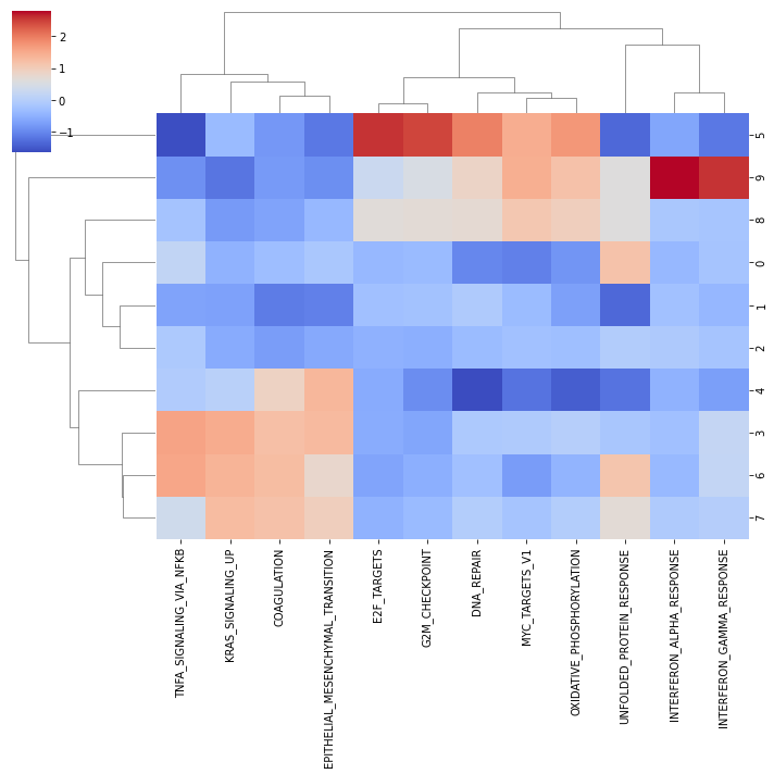
And visualize them:

[30]:

sns.clustermap(mean_acts, xticklabels=mean_acts.columns, cmap='coolwarm', z_score=1)
plt.show()

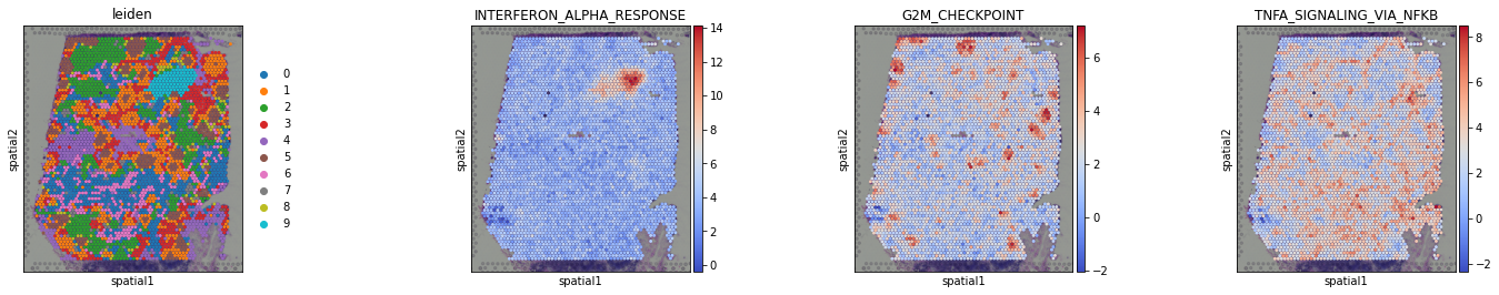
We can visualize again on the tissue some cluster-specific terms:

[31]:

sc.pl.spatial(acts, color=['leiden', 'INTERFERON_ALPHA_RESPONSE', 'G2M_CHECKPOINT', 'TNFA_SIGNALING_VIA_NFKB'], cmap='coolwarm', size=1.5, wspace=0)