Transcription factor activity inference
scRNA-seq yield many molecular readouts that are hard to interpret by themselves. One way of summarizing this information is by infering transcription factor (TF) activities from prior knowledge.
In this notebook we showcase how to use decoupler for TF activity inference with the 3k PBMCs 10X data-set. The data consists of 3k PBMCs from a Healthy Donor and is freely available from 10x Genomics here from this webpage
Note
This tutorial assumes that you already know the basics of decoupler. Else, check out the Usage tutorial first.
Loading packages
First, we need to load the relevant packages, scanpy to handle scRNA-seq data and decoupler to use statistical methods.
[1]:
import scanpy as sc
import decoupler as dc

# Plotting options, change to your liking
sc.settings.set_figure_params(dpi=200, frameon=False)
sc.set_figure_params(dpi=200)
sc.set_figure_params(figsize=(4, 4))
Loading the data
We can download the data easily using scanpy:
[2]:
adata = sc.datasets.pbmc3k_processed()
adata
[2]:
AnnData object with n_obs × n_vars = 2638 × 1838
    obs: 'n_genes', 'percent_mito', 'n_counts', 'louvain'
    var: 'n_cells'
    uns: 'draw_graph', 'louvain', 'louvain_colors', 'neighbors', 'pca', 'rank_genes_groups'
    obsm: 'X_pca', 'X_tsne', 'X_umap', 'X_draw_graph_fr'
    varm: 'PCs'
    obsp: 'distances', 'connectivities'
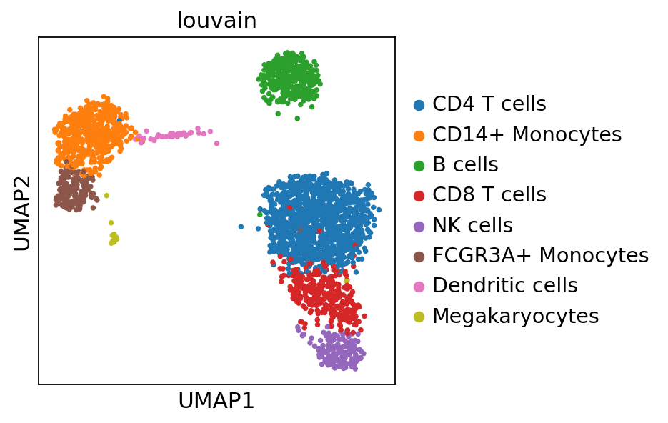
We can visualize the different cell types in it:
[3]:
sc.pl.umap(adata, color='louvain')
CollecTRI network
CollecTRI is a comprehensive resource containing a curated collection of TFs and their transcriptional targets compiled from 12 different resources. This collection provides an increased coverage of transcription factors and a superior performance in identifying perturbed TFs compared to our previous DoRothEA network and other literature based GRNs. Similar to DoRothEA, interactions are weighted by their mode of regulation (activation or inhibition).
For this example we will use the human version (mouse and rat are also available). We can use decoupler to retrieve it from omnipath. The argument split_complexes keeps complexes or splits them into subunits, by default we recommend to keep complexes together.
[4]:
net = dc.get_collectri(organism='human', split_complexes=False)
net
[4]:
| source | target | weight | PMID | |
|---|---|---|---|---|
| 0 | MYC | TERT | 1 | 10022128;10491298;10606235;10637317;10723141;1... |
| 1 | SPI1 | BGLAP | 1 | 10022617 |
| 2 | SMAD3 | JUN | 1 | 10022869;12374795 |
| 3 | SMAD4 | JUN | 1 | 10022869;12374795 |
| 4 | STAT5A | IL2 | 1 | 10022878;11435608;17182565;17911616;22854263;2... |
| ... | ... | ... | ... | ... |
| 43173 | NFKB | hsa-miR-143-3p | 1 | 19472311 |
| 43174 | AP1 | hsa-miR-206 | 1 | 19721712 |
| 43175 | NFKB | hsa-miR-21-5p | 1 | 20813833;22387281 |
| 43176 | NFKB | hsa-miR-224-5p | 1 | 23474441;23988648 |
| 43177 | AP1 | hsa-miR-144 | 1 | 23546882 |
43178 rows × 4 columns
Note
In this tutorial we use the network CollecTRI, but we could use any other GRN coming from an inference method such as CellOracle, pySCENIC or SCENIC+.
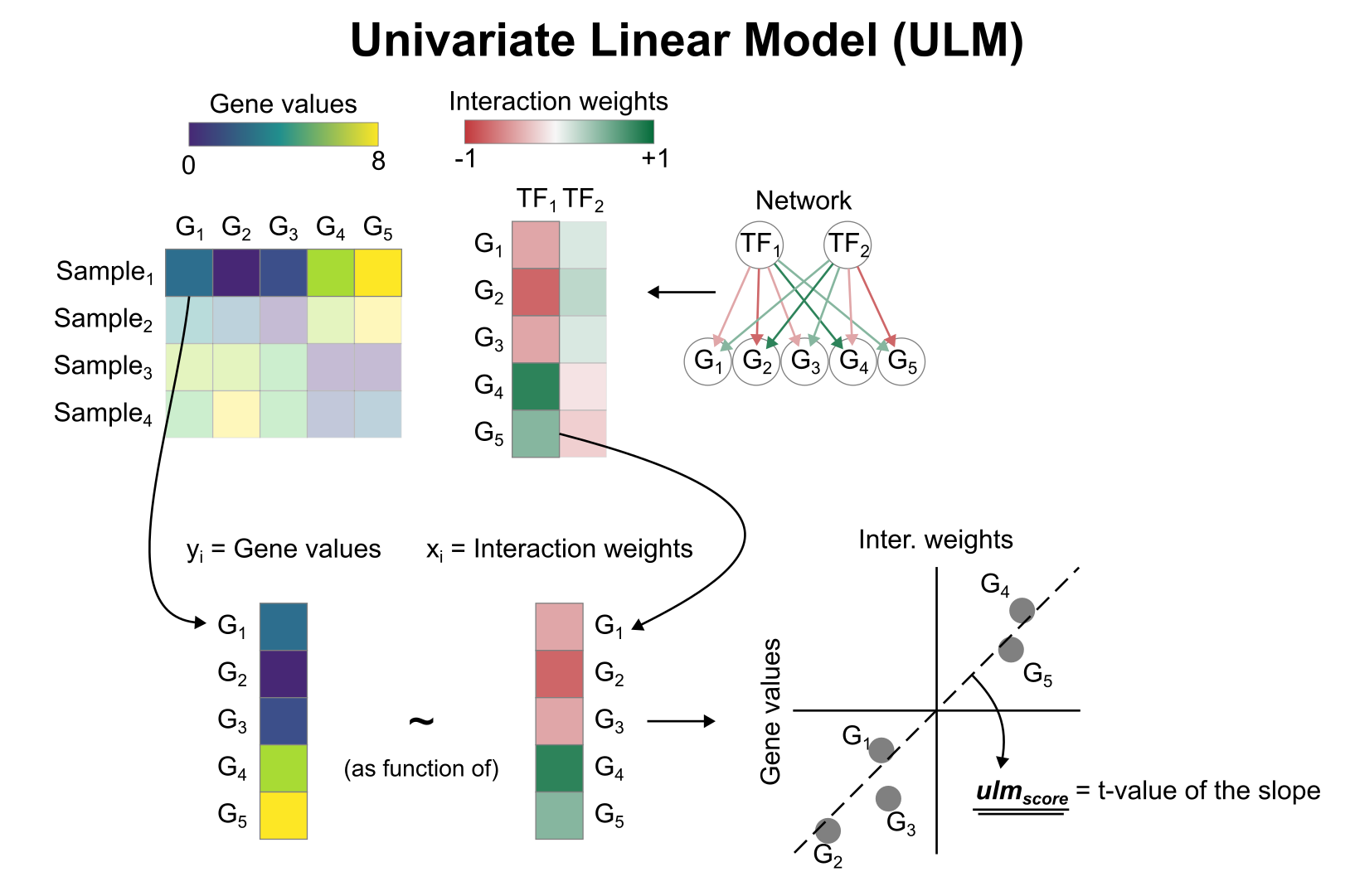
Activity inference with univariate linear model (ULM)
To infer TF enrichment scores we will run the univariate linear model (ulm) method. For each cell in our dataset (adata) and each TF in our network (net), it fits a linear model that predicts the observed gene expression based solely on the TF’s TF-Gene interaction weights. Once fitted, the obtained t-value of the slope is the score. If it is positive, we interpret that the TF is active and if it is negative we interpret that it is inactive.
To run decoupler methods, we need an input matrix (mat), an input prior knowledge network/resource (net), and the name of the columns of net that we want to use.
[5]:
dc.run_ulm(
    mat=adata,
    net=net,
    source='source',
    target='target',
    weight='weight',
    verbose=True
)
1 features of mat are empty, they will be removed.
Running ulm on mat with 2638 samples and 13713 targets for 608 sources.
100%|███████████████████████████████████████████████████████████████████████████████████████████████████████████████████████████| 1/1 [00:00<00:00, 1.93it/s]
The obtained scores (ulm_estimate) and p-values (ulm_pvals) are stored in the .obsm key:
[6]:
adata.obsm['ulm_estimate']
[6]:
| ABL1 | AHR | AIRE | AP1 | APEX1 | AR | ARID1A | ARID1B | ARID3A | ARID3B | ... | ZNF362 | ZNF382 | ZNF384 | ZNF395 | ZNF436 | ZNF699 | ZNF76 | ZNF804A | ZNF91 | ZXDC | |
|---|---|---|---|---|---|---|---|---|---|---|---|---|---|---|---|---|---|---|---|---|---|
| AAACATACAACCAC-1 | 3.105468 | 0.879592 | 2.909616 | 3.406131 | 0.822555 | 2.255649 | 0.622126 | -0.454210 | -0.497625 | -0.454210 | ... | 0.051970 | -3.070555 | -0.287258 | -0.454214 | 0.485032 | -1.168097 | 0.816615 | -0.090827 | 1.496588 | 2.328766 |
| AAACATTGAGCTAC-1 | 0.644366 | -0.912154 | 0.994992 | 2.265793 | 0.947906 | 1.649951 | -0.594850 | -0.594846 | -0.651707 | -0.594846 | ... | -0.334580 | 0.798244 | 0.266120 | 0.217652 | -0.651681 | -0.263382 | 1.700061 | -0.118951 | 2.089825 | 0.693020 |
| AAACATTGATCAGC-1 | 2.105423 | 2.411347 | 2.517772 | 5.470295 | 2.126797 | 3.830123 | -0.566923 | -0.566920 | -0.621111 | 0.393613 | ... | -0.841067 | -5.552263 | 0.400812 | 0.393611 | -0.621086 | -0.214621 | -0.206983 | 1.408917 | 1.648628 | 0.393655 |
| AAACCGTGCTTCCG-1 | 0.276449 | -0.050781 | 3.699017 | 3.061379 | 2.169211 | 4.214366 | -0.523785 | -0.523782 | -0.573849 | -0.523782 | ... | 2.882433 | -0.057149 | -0.331257 | -0.523789 | 0.356896 | 0.639145 | 0.739300 | -0.104740 | 3.708728 | 2.535483 |
| AAACCGTGTATGCG-1 | 2.003766 | -0.067349 | 2.869071 | 3.876005 | 2.185347 | 1.854994 | -0.393699 | 1.259139 | -0.431328 | -0.393696 | ... | 1.182478 | 0.528311 | 1.057657 | 2.912763 | -0.431311 | 2.207839 | -0.143738 | -0.078726 | 2.713175 | -0.393741 |
| ... | ... | ... | ... | ... | ... | ... | ... | ... | ... | ... | ... | ... | ... | ... | ... | ... | ... | ... | ... | ... | ... |
| TTTCGAACTCTCAT-1 | 2.286176 | 1.772627 | 3.793108 | 3.976223 | 1.279253 | 4.544536 | 0.336520 | -0.569478 | 0.203251 | 0.336517 | ... | 1.184737 | -2.550669 | -0.360157 | -0.569485 | -0.623888 | 0.154066 | -0.207928 | 0.792007 | 3.299084 | 1.534470 |
| TTTCTACTGAGGCA-1 | 2.274223 | 0.702174 | 1.214197 | 2.498593 | 0.813810 | 3.195549 | 0.318464 | -0.589052 | 0.183192 | 0.318462 | ... | 0.350057 | -1.457127 | -0.372536 | -0.589059 | -0.645333 | -0.807615 | -0.215074 | 0.789607 | 2.952728 | 1.226170 |
| TTTCTACTTCCTCG-1 | 2.906737 | 1.537232 | 2.975087 | 2.567488 | 0.765529 | 1.361353 | -0.415441 | -0.415438 | -0.455148 | -0.415438 | ... | -0.616327 | -2.878397 | -0.262738 | -0.415443 | -0.455130 | -0.583188 | -0.151677 | -0.083074 | 1.635638 | -0.415485 |
| TTTGCATGAGAGGC-1 | -0.308224 | 0.795947 | 2.813390 | 3.779697 | 3.331115 | 0.986302 | -0.363216 | -0.363214 | -0.397933 | -0.363214 | ... | 0.543865 | 0.487409 | -0.229710 | -0.363219 | -0.397917 | -0.308451 | -0.132609 | -0.072632 | 3.547983 | 1.242570 |
| TTTGCATGCCTCAC-1 | 1.273584 | 0.915988 | 2.149884 | 3.688747 | 1.150673 | 1.625602 | -0.442853 | -0.442850 | -0.485181 | -0.442851 | ... | 0.129370 | -2.014078 | -0.280075 | -0.442855 | 0.579456 | -0.684479 | -0.161685 | -1.254577 | 1.927536 | 1.889836 |
2638 rows × 608 columns
Note: Each run of run_ulm overwrites what is inside of ulm_estimate and ulm_pvals. if you want to run ulm with other resources and still keep the activities inside the same AnnData object, you can store the results in any other key in .obsm with different names, for example:
[7]:
adata.obsm['collectri_ulm_estimate'] = adata.obsm['ulm_estimate'].copy()
adata.obsm['collectri_ulm_pvals'] = adata.obsm['ulm_pvals'].copy()
adata
[7]:
AnnData object with n_obs × n_vars = 2638 × 1838
    obs: 'n_genes', 'percent_mito', 'n_counts', 'louvain'
    var: 'n_cells'
    uns: 'draw_graph', 'louvain', 'louvain_colors', 'neighbors', 'pca', 'rank_genes_groups'
    obsm: 'X_pca', 'X_tsne', 'X_umap', 'X_draw_graph_fr', 'ulm_estimate', 'ulm_pvals', 'collectri_ulm_estimate', 'collectri_ulm_pvals'
    varm: 'PCs'
    obsp: 'distances', 'connectivities'
Visualization
To visualize the obtained scores, we can re-use many of scanpy’s plotting functions. First though, we need to extract them from the adata object.
[8]:
acts = dc.get_acts(adata, obsm_key='ulm_estimate')
acts
[8]:
AnnData object with n_obs × n_vars = 2638 × 608
    obs: 'n_genes', 'percent_mito', 'n_counts', 'louvain'
    uns: 'draw_graph', 'louvain', 'louvain_colors', 'neighbors', 'pca', 'rank_genes_groups'
    obsm: 'X_pca', 'X_tsne', 'X_umap', 'X_draw_graph_fr', 'ulm_estimate', 'ulm_pvals', 'collectri_ulm_estimate', 'collectri_ulm_pvals'
dc.get_acts returns a new AnnData object which holds the obtained activities in its .X attribute, allowing us to re-use many scanpy functions, for example:
[9]:
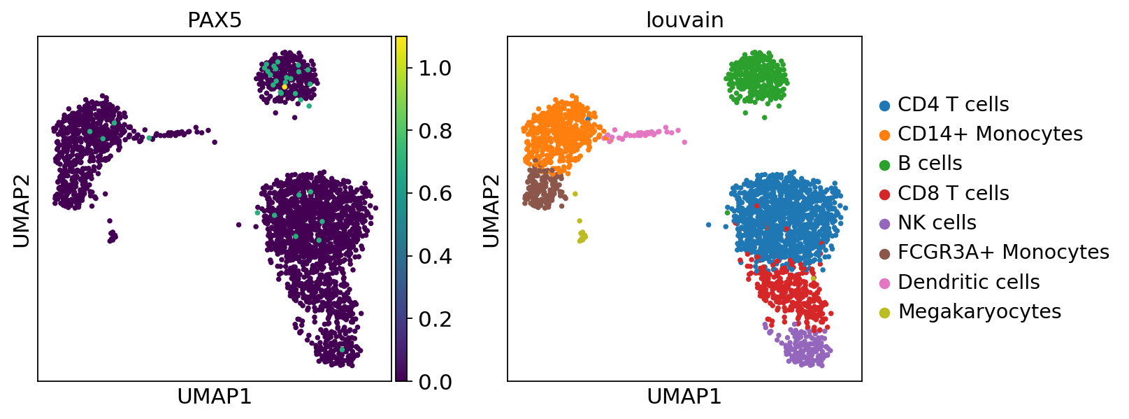
sc.pl.umap(acts, color=['PAX5', 'louvain'], cmap='RdBu_r', vcenter=0)
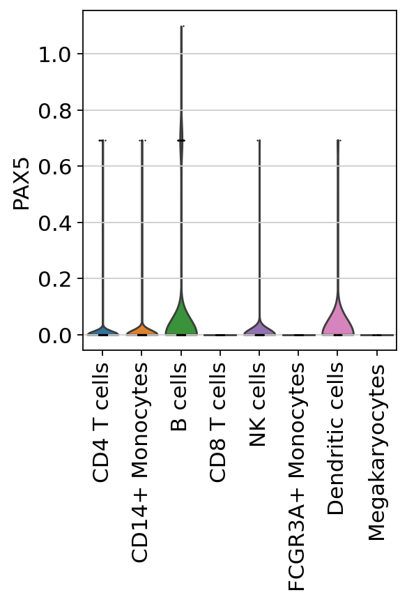
sc.pl.violin(acts, keys=['PAX5'], groupby='louvain', rotation=90)
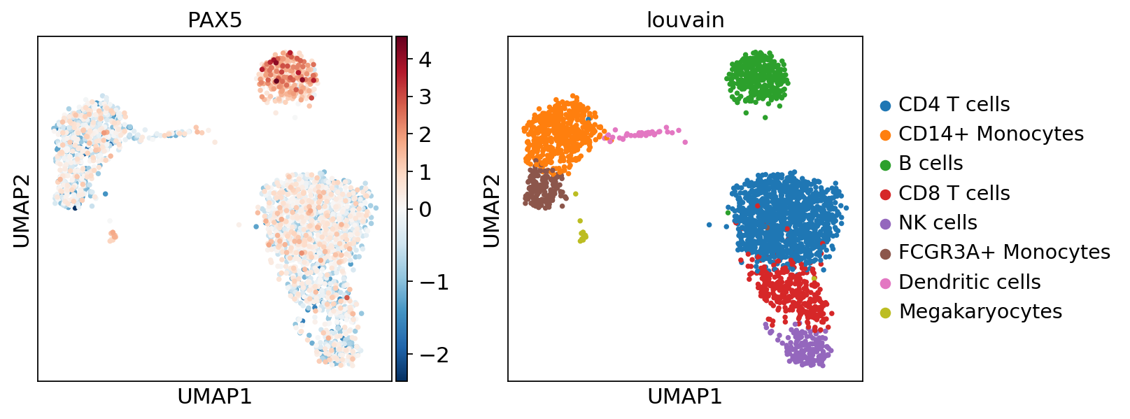
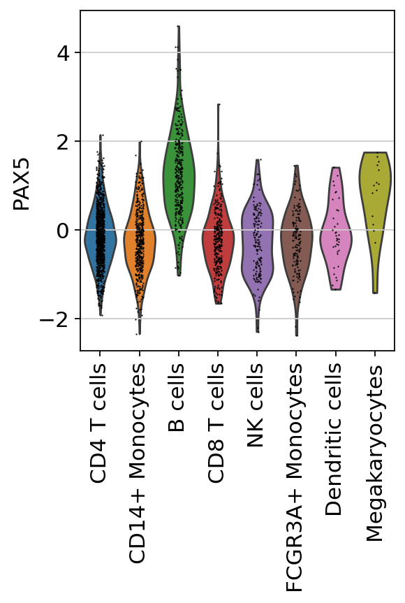
Here we observe the activity infered for PAX5 across cells, which it is particulary active in B cells. Interestingly, PAX5 is a known TF crucial for B cell identity and function. The inference of activities from “foot-prints” of target genes is more informative than just looking at the molecular readouts of a given TF, as an example here is the gene expression of PAX5, which is not very informative by itself since it is just expressed in few cells:
[10]:
sc.pl.umap(adata, color=['PAX5', 'louvain'])
sc.pl.violin(adata, keys=['PAX5'], groupby='louvain', rotation=90)
Exploration
Let’s identify which are the top TF per cell type. We can do it by using the function dc.rank_sources_groups, which identifies marker TFs using the same statistical tests available in scanpy’s scanpy.tl.rank_genes_groups.
[11]:
df = dc.rank_sources_groups(acts, groupby='louvain', reference='rest', method='t-test_overestim_var')
df
[11]:
| group | reference | names | statistic | meanchange | pvals | pvals_adj | |
|---|---|---|---|---|---|---|---|
| 0 | B cells | rest | EBF1 | 46.169485 | 2.599952 | 7.623835e-180 | 1.158823e-177 |
| 1 | B cells | rest | RFXANK | 41.651199 | 10.032308 | 1.121601e-186 | 6.819333e-184 |
| 2 | B cells | rest | RFXAP | 41.465602 | 10.624727 | 1.992744e-185 | 4.038627e-183 |
| 3 | B cells | rest | RFX5 | 41.407184 | 8.863535 | 1.182159e-185 | 3.593764e-183 |
| 4 | B cells | rest | CIITA | 38.505500 | 6.445218 | 7.559868e-173 | 9.192799e-171 |
| ... | ... | ... | ... | ... | ... | ... | ... |
| 4859 | NK cells | rest | TGFB1I1 | -11.229069 | -1.846338 | 1.387798e-24 | 4.218906e-23 |
| 4860 | NK cells | rest | HMGA2 | -11.360268 | -1.685328 | 5.055666e-25 | 1.707692e-23 |
| 4861 | NK cells | rest | MYC | -11.377993 | -2.238815 | 6.106139e-25 | 1.953964e-23 |
| 4862 | NK cells | rest | THRA | -11.795926 | -1.196717 | 2.315007e-26 | 8.797027e-25 |
| 4863 | NK cells | rest | TCF4 | -11.821820 | -1.300579 | 8.805137e-27 | 3.569016e-25 |
4864 rows × 7 columns
We can then extract the top 3 markers per cell type:
[12]:
n_markers = 3
source_markers = df.groupby('group').head(n_markers).groupby('group')['names'].apply(lambda x: list(x)).to_dict()
source_markers
[12]:
{'B cells': ['EBF1', 'RFXANK', 'RFXAP'],
 'CD14+ Monocytes': ['ONECUT1', 'EHF', 'ELF3'],
 'CD4 T cells': ['ZBTB4', 'MYC', 'ZBED1'],
 'CD8 T cells': ['KLF13', 'NFKB2', 'RELB'],
 'Dendritic cells': ['RFXAP', 'RFXANK', 'RFX5'],
 'FCGR3A+ Monocytes': ['SIN3A', 'PPARD', 'SPIC'],
 'Megakaryocytes': ['PKNOX1', 'PBX2', 'FLI1'],
 'NK cells': ['ZGLP1', 'CEBPZ', 'ZNF395']}
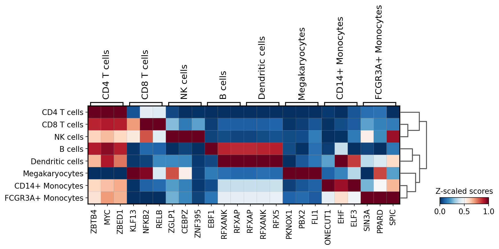
We can plot the obtained markers:
[13]:
sc.pl.matrixplot(acts, source_markers, 'louvain', dendrogram=True, standard_scale='var',
                 colorbar_title='Z-scaled scores', cmap='RdBu_r')
WARNING: dendrogram data not found (using key=dendrogram_louvain). Running `sc.tl.dendrogram` with default parameters. For fine tuning it is recommended to run `sc.tl.dendrogram` independently.
We can check individual TFs by plotting their distributions:
[14]:
sc.pl.violin(acts, keys=['EBF1'], groupby='louvain', rotation=90)
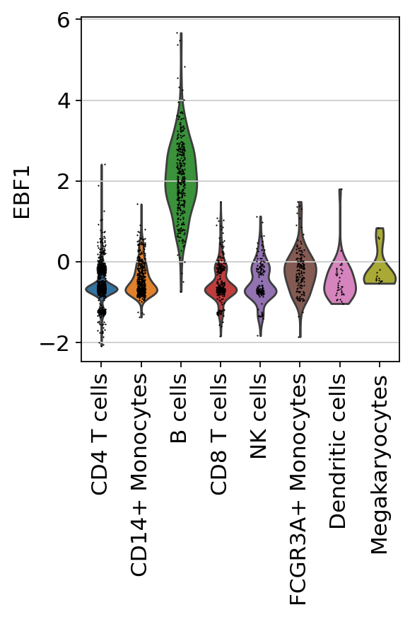
Here we can observe the TF activities for EBF1, which is a known marker TF for B cells.
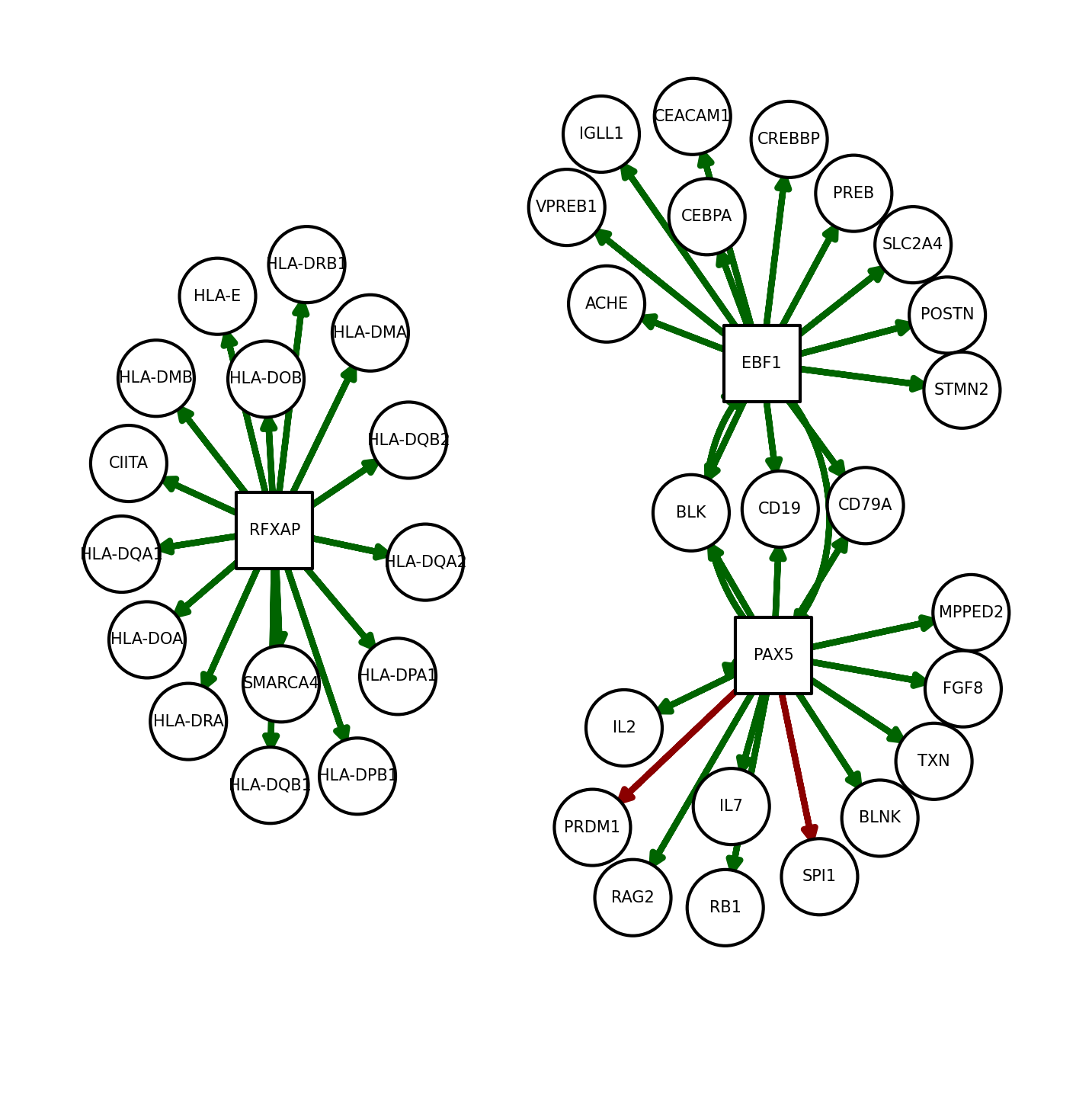
We can also plot net to see relevant TFs and target genes:
[15]:
dc.plot_network(
    net=net,
    n_sources=['PAX5', 'EBF1', 'RFXAP'],
    n_targets=15,
    node_size=100,
    s_cmap='white',
    t_cmap='white',
    c_pos_w='darkgreen',
    c_neg_w='darkred',
    figsize=(5, 5)
)
Note
If your data consist of different conditions with enough samples, we recommend to work with pseudo-bulk profiles instead. Check this vignette for more informatin.