Spatial functional analysis
Spatial transcriptomics technologies yield many molecular readouts that are hard to interpret by themselves. One way of summarizing this information is by inferring biological activities from prior knowledge.
In this notebook we showcase how to use decoupler for transcription factor and pathway activity inference from a human data-set. The data consists of a 10X Genomics Visium slide of a human lymph node and it is available at their website.
Note
This tutorial assumes that you already know the basics of decoupler. Else, check out the Usage tutorial first.
Loading packages
First, we need to load the relevant packages, scanpy to handle RNA-seq data and decoupler to use statistical methods.
[1]:
import scanpy as sc
import decoupler as dc

# Only needed for processing
import numpy as np
import pandas as pd

# Plotting options, change to your liking
sc.settings.set_figure_params(dpi=200, frameon=False)
sc.set_figure_params(dpi=200)
sc.set_figure_params(figsize=(4, 4))
Loading the data
We can download the data easily using scanpy:
[2]:
adata = sc.datasets.visium_sge(sample_id="V1_Human_Lymph_Node")
adata.var_names_make_unique()
adata
[2]:
AnnData object with n_obs × n_vars = 4035 × 36601
    obs: 'in_tissue', 'array_row', 'array_col'
    var: 'gene_ids', 'feature_types', 'genome'
    uns: 'spatial'
    obsm: 'spatial'
QC, projection and clustering
Here we follow the standard pre-processing steps as described in the scanpy vignette. These steps carry out the selection and filtration of spots based on quality control metrics and data normalization.
Note
This is just an example, these steps should change depending on the data.
[3]:
# Basic filtering
sc.pp.filter_cells(adata, min_genes=200)
sc.pp.filter_genes(adata, min_cells=10)

# Normalize the data
sc.pp.normalize_total(adata, target_sum=1e4)
sc.pp.log1p(adata)
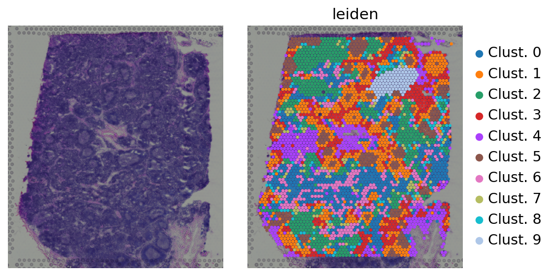
Then we group spots based on the similarity of their transcription profiles. We can visualize the obtained clusters on a UMAP or directly at the tissue:
[4]:
# Store norm counts
adata.layers['log_norm'] = adata.X.copy()

# Identify highly variable genes
sc.pp.highly_variable_genes(adata)

# Scale the data
sc.pp.scale(adata, max_value=10)

# Generate PCA features
sc.tl.pca(adata, svd_solver='arpack')

# Restore X to be norm counts
dc.swap_layer(adata, 'log_norm', X_layer_key=None, inplace=True)

# Compute distances in the PCA space, and find spot neighbors
sc.pp.neighbors(adata)

# Run leiden clustering algorithm
sc.tl.leiden(adata)
adata.obs['leiden'] = ['Clust. {0}'.format(i) for i in adata.obs['leiden']]
[5]:
sc.pl.spatial(adata, color=[None, 'leiden'], size=1.5, wspace=0, frameon=False)
Spatial Connectivity
Additionally, we can incorporate spatial information in our analyses by accounting for the spatial connectivity of our observations (in this case spots). By weighting the spatial proximity of our spots to the neighboring ones, we can transform our data to incorporate spatial context.
Note
This section is optional, it is also valid to compute enrichment scores without taking into account the spatial component.
To generate spatial weights based on spatial proximity we will use liana. More information is available in this vignette.
[6]:
import liana as li

li.ut.spatial_neighbors(
    adata,
    bandwidth=150,
    cutoff=0.1,
    kernel='gaussian',
    set_diag=True,
    standardize=True
)
[7]:
# Plot the spatial weights of one spot in our object
adata.obs['conn'] = adata.obsp['spatial_connectivities'][0].A.ravel()
sc.pl.spatial(adata, color='conn', size=1.5, frameon=False)
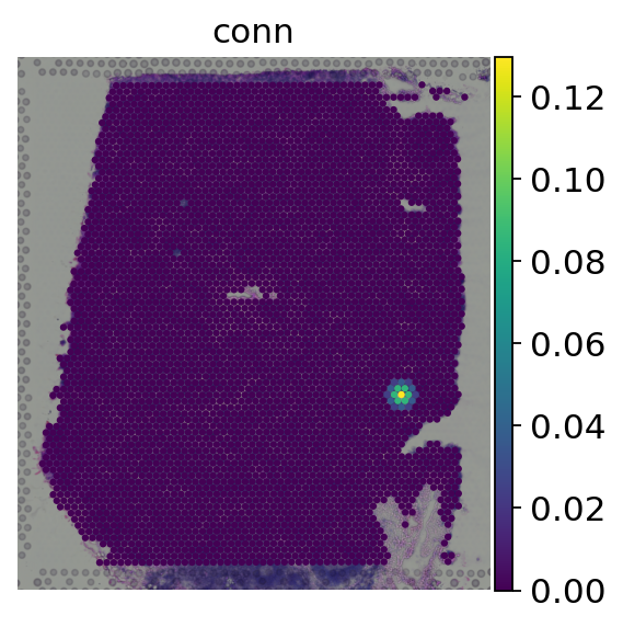
We can see that for a given spot, the spatial weight is at its maximum on itself and decreases the more distant other spots are. Now we can spatially weight the gene expression values:
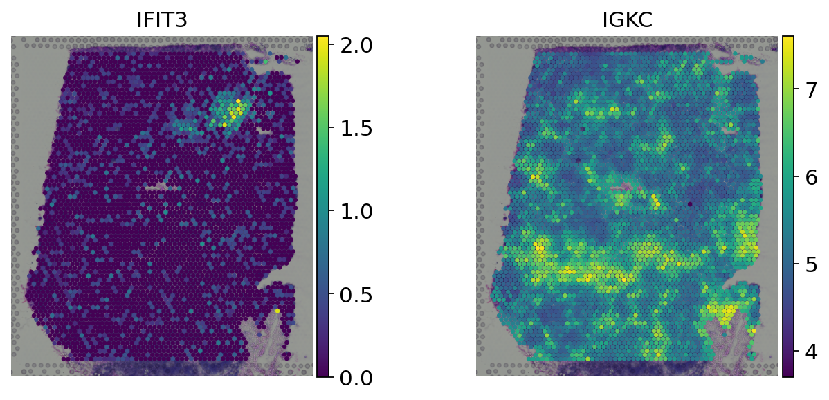
[8]:
# Update X with spatially weighted gene exression
adata.X = adata.obsp['spatial_connectivities'].A.dot(adata.X.A)
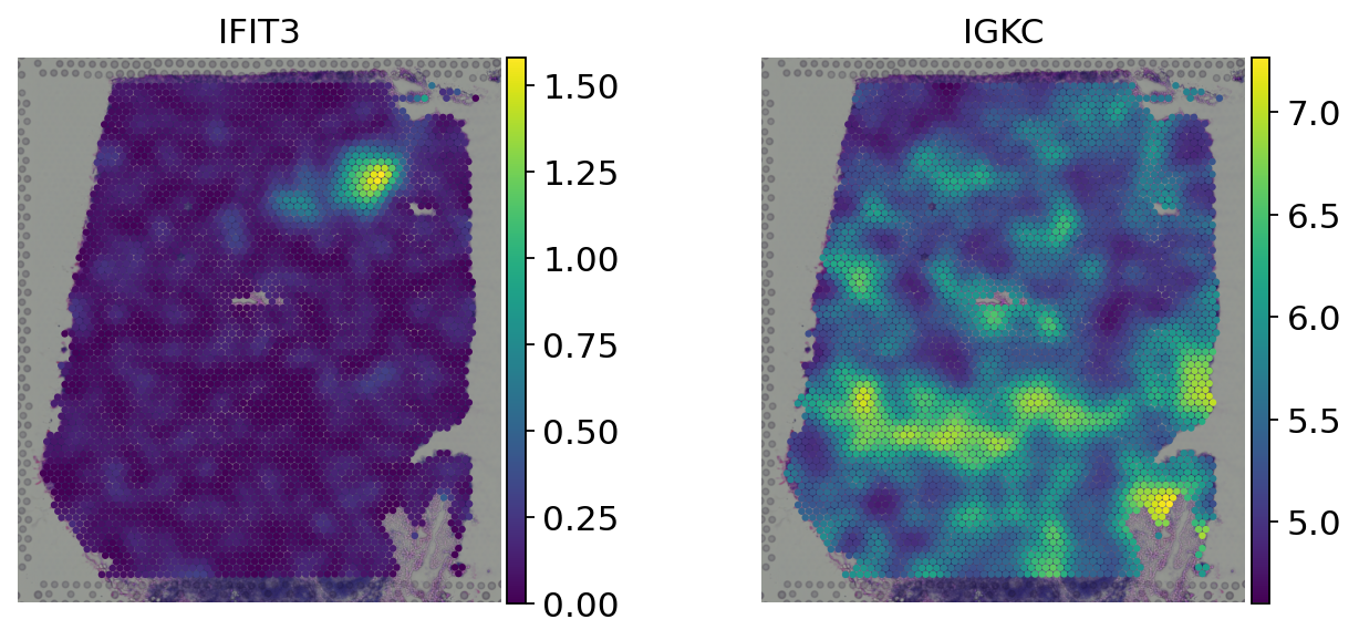
We can plot the original log-normalized counts with the new spatialy transformed values:
[9]:
genes = ['IFIT3', 'IGKC']

# Log-normalized counts
sc.pl.spatial(adata, color=genes, size=1.5, frameon=False, layer='log_norm')

# Spatially weighted gene expression
sc.pl.spatial(adata, color=genes, size=1.5, frameon=False)
Transcription factor activity inference
The first functional analysis we can perform is to infer transcription factor (TF) activities from our transcriptomics data. We will need a gene regulatory network (GRN) and a statistical method.
CollecTRI network
CollecTRI is a comprehensive resource containing a curated collection of TFs and their transcriptional targets compiled from 12 different resources. This collection provides an increased coverage of transcription factors and a superior performance in identifying perturbed TFs compared to our previous DoRothEA network and other literature based GRNs. Similar to DoRothEA, interactions are weighted by their mode of regulation (activation or inhibition).
For this example we will use the human version (mouse and rat are also available). We can use decoupler to retrieve it from omnipath. The argument split_complexes keeps complexes or splits them into subunits, by default we recommend to keep complexes together.
Note
In this tutorial we use the network CollecTRI, but we could use any other GRN coming from an inference method such as CellOracle, pySCENIC or SCENIC+.
[10]:
net = dc.get_collectri(organism='human', split_complexes=False)
net
Downloading data from `https://omnipathdb.org/queries/enzsub?format=json`
Downloading data from `https://omnipathdb.org/queries/interactions?format=json`
Downloading data from `https://omnipathdb.org/queries/complexes?format=json`
Downloading data from `https://omnipathdb.org/queries/annotations?format=json`
Downloading data from `https://omnipathdb.org/queries/intercell?format=json`
Downloading data from `https://omnipathdb.org/about?format=text`
[10]:
| source | target | weight | PMID | |
|---|---|---|---|---|
| 0 | MYC | TERT | 1 | 10022128;10491298;10606235;10637317;10723141;1... |
| 1 | SPI1 | BGLAP | 1 | 10022617 |
| 2 | SMAD3 | JUN | 1 | 10022869;12374795 |
| 3 | SMAD4 | JUN | 1 | 10022869;12374795 |
| 4 | STAT5A | IL2 | 1 | 10022878;11435608;17182565;17911616;22854263;2... |
| ... | ... | ... | ... | ... |
| 43173 | NFKB | hsa-miR-143-3p | 1 | 19472311 |
| 43174 | AP1 | hsa-miR-206 | 1 | 19721712 |
| 43175 | NFKB | hsa-miR-21-5p | 1 | 20813833;22387281 |
| 43176 | NFKB | hsa-miR-224-5p | 1 | 23474441;23988648 |
| 43177 | AP1 | hsa-miR-144 | 1 | 23546882 |
43178 rows × 4 columns
Activity inference with Univariate Linear Model (ULM)
To infer TF enrichment scores we will run the Univariate Linear Model (ulm) method. For each spot in our slide (adata) and each TF in our network (net), it fits a linear model that predicts the observed gene expression based solely on the TF’s TF-Gene interaction weights. Once fitted, the obtained t-value of the slope is the score. If it is positive, we interpret that the TF is active and if it is negative we interpret that it is inactive.
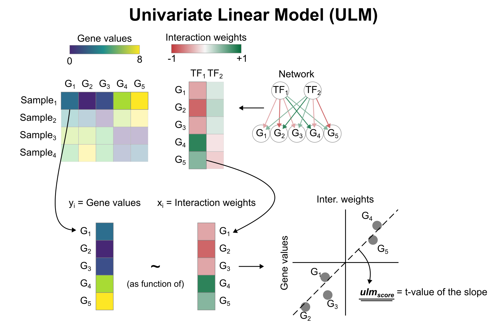
To run decoupler methods, we need an input matrix (mat), an input prior knowledge network/resource (net), and the name of the columns of net that we want to use.
[11]:
dc.run_ulm(
    mat=adata,
    net=net,
    source='source',
    target='target',
    weight='weight',
    verbose=True,
    use_raw=False
)
Running ulm on mat with 4032 samples and 19813 targets for 714 sources.
The obtained scores (ulm_estimate) and p-values (ulm_pvals) are stored in the .obsm key:
[12]:
adata.obsm['ulm_estimate']
[12]:
| ABL1 | AHR | AIP | AIRE | AP1 | APEX1 | AR | ARID1A | ARID1B | ARID3A | ... | ZNF382 | ZNF384 | ZNF395 | ZNF423 | ZNF436 | ZNF699 | ZNF76 | ZNF804A | ZNF91 | ZXDC | |
|---|---|---|---|---|---|---|---|---|---|---|---|---|---|---|---|---|---|---|---|---|---|
| AAACAAGTATCTCCCA-1 | 2.506540 | 2.993418 | -0.224612 | 1.088716 | 8.932042 | 3.467653 | 8.088826 | 0.097465 | 1.640161 | 1.590863 | ... | -2.141593 | 0.041473 | 0.137326 | -1.132138 | 1.519211 | 2.201835 | 0.106273 | -0.554477 | 1.577712 | 5.126571 |
| AAACAATCTACTAGCA-1 | 1.861013 | 2.003174 | -0.234753 | 0.840002 | 7.381738 | 2.214163 | 7.312593 | -0.160331 | 1.457745 | 0.701439 | ... | -1.719987 | -0.552122 | -0.236105 | -1.066291 | 1.508229 | 1.620679 | 0.599542 | -0.930530 | 1.557906 | 4.704382 |
| AAACACCAATAACTGC-1 | 2.365444 | 3.012575 | -0.247704 | 1.302476 | 9.036439 | 3.478431 | 8.182927 | 0.190212 | 1.234260 | 1.334810 | ... | -1.935273 | -0.352290 | 0.110648 | -1.090288 | 1.026727 | 2.036324 | 0.634918 | -0.373306 | 2.066460 | 4.922176 |
| AAACAGAGCGACTCCT-1 | 1.333631 | 3.089248 | -0.161767 | 1.122681 | 8.437885 | 3.095499 | 7.818810 | -0.074081 | 2.859876 | 2.275510 | ... | -1.949705 | -0.472413 | 1.141847 | -1.144544 | 1.538650 | 1.718085 | 1.172972 | 0.167259 | 1.726077 | 4.207001 |
| AAACAGCTTTCAGAAG-1 | 1.444055 | 2.606838 | -0.424777 | 0.746851 | 7.309249 | 3.678788 | 6.895603 | -0.038943 | 2.916240 | 2.473541 | ... | -1.677928 | -0.270460 | -0.091756 | -1.113962 | 0.842817 | 1.549942 | 0.918052 | 0.020900 | 1.605347 | 4.549479 |
| ... | ... | ... | ... | ... | ... | ... | ... | ... | ... | ... | ... | ... | ... | ... | ... | ... | ... | ... | ... | ... | ... |
| TTGTTTCACATCCAGG-1 | 2.178375 | 2.633951 | -0.171126 | 0.774759 | 9.022694 | 3.937260 | 7.809430 | 0.121977 | 1.853033 | 1.935024 | ... | -1.907115 | -0.074763 | -0.093024 | -1.062878 | 1.136265 | 1.897447 | 0.283017 | -0.189876 | 1.996677 | 5.542336 |
| TTGTTTCATTAGTCTA-1 | 2.148535 | 3.249435 | -0.164014 | 1.266401 | 9.157030 | 3.788883 | 8.210668 | -0.031493 | 1.914353 | 1.334394 | ... | -1.997858 | -0.149779 | -0.424333 | -1.120992 | 1.545704 | 2.204408 | 0.580634 | -0.393936 | 2.131220 | 5.359280 |
| TTGTTTCCATACAACT-1 | 2.471877 | 3.029328 | 0.003349 | 1.515853 | 9.260170 | 3.733936 | 8.150513 | 0.272917 | 2.101049 | 1.329936 | ... | -2.033781 | -0.252704 | -0.093840 | -1.051247 | 1.592259 | 1.741617 | 0.421107 | -0.850126 | 1.839918 | 5.194634 |
| TTGTTTGTATTACACG-1 | 2.095661 | 2.986843 | -0.117071 | 1.187332 | 9.163303 | 3.595011 | 7.863039 | 0.219370 | 1.258791 | 1.072886 | ... | -2.060137 | -0.159512 | 0.151495 | -1.038933 | 1.136436 | 1.912966 | 0.376731 | -0.870485 | 2.227823 | 5.392848 |
| TTGTTTGTGTAAATTC-1 | 1.798320 | 2.622384 | -0.314093 | 1.126644 | 8.291216 | 2.921452 | 7.545118 | -0.136264 | 1.678849 | 1.517110 | ... | -1.643596 | -0.724133 | -0.226429 | -1.170998 | 1.248425 | 1.649105 | 0.851030 | -0.691052 | 1.609469 | 4.503331 |
4032 rows × 714 columns
Note: Each run of run_ulm overwrites what is inside of ulm_estimate and ulm_pvals. if you want to run ulm with other resources and still keep the activities inside the same AnnData object, you can store the results in any other key in .obsm with different names, for example:
[13]:
adata.obsm['collectri_ulm_estimate'] = adata.obsm['ulm_estimate'].copy()
adata.obsm['collectri_ulm_pvals'] = adata.obsm['ulm_pvals'].copy()
adata
[13]:
AnnData object with n_obs × n_vars = 4032 × 19813
    obs: 'in_tissue', 'array_row', 'array_col', 'n_genes', 'leiden', 'conn'
    var: 'gene_ids', 'feature_types', 'genome', 'n_cells', 'highly_variable', 'means', 'dispersions', 'dispersions_norm', 'mean', 'std'
    uns: 'spatial', 'log1p', 'hvg', 'pca', 'neighbors', 'leiden', 'leiden_colors'
    obsm: 'spatial', 'X_pca', 'ulm_estimate', 'ulm_pvals', 'collectri_ulm_estimate', 'collectri_ulm_pvals'
    varm: 'PCs'
    layers: 'log_norm'
    obsp: 'distances', 'connectivities', 'spatial_connectivities'
Visualization
To visualize the obtained scores, we can re-use many of scanpy’s plotting functions. First though, we need to extract them from the adata object.
[14]:
acts = dc.get_acts(adata, obsm_key='collectri_ulm_estimate')
acts
[14]:
AnnData object with n_obs × n_vars = 4032 × 714
    obs: 'in_tissue', 'array_row', 'array_col', 'n_genes', 'leiden', 'conn'
    uns: 'spatial', 'log1p', 'hvg', 'pca', 'neighbors', 'leiden', 'leiden_colors'
    obsm: 'spatial', 'X_pca', 'ulm_estimate', 'ulm_pvals', 'collectri_ulm_estimate', 'collectri_ulm_pvals'
dc.get_acts returns a new AnnData object which holds the obtained activities in its .X attribute, allowing us to re-use many scanpy functions, for example:
[15]:
sc.pl.spatial(
    acts,
    color=['IRF1', 'leiden'],
    cmap='RdBu_r',
    size=1.5,
    vcenter=0,
    frameon=False
)
sc.pl.violin(
    acts,
    keys='IRF1',
    groupby='leiden',
    rotation=90
)
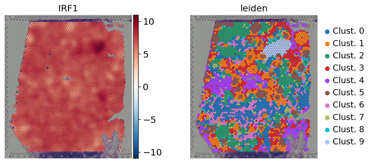
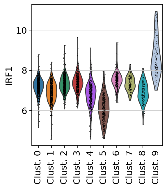
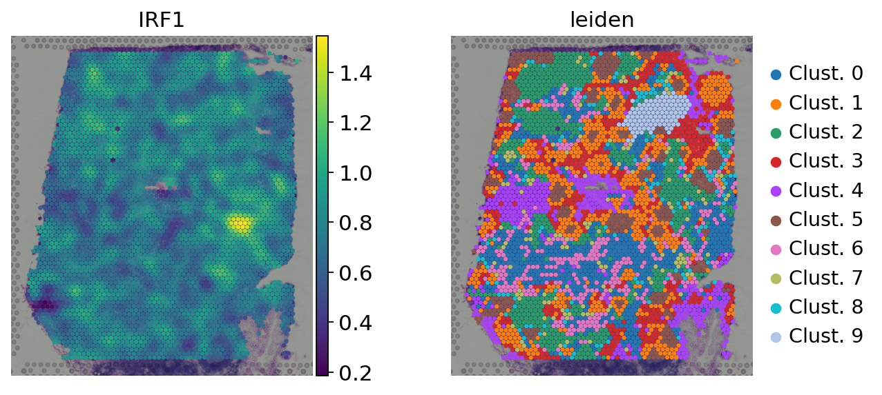
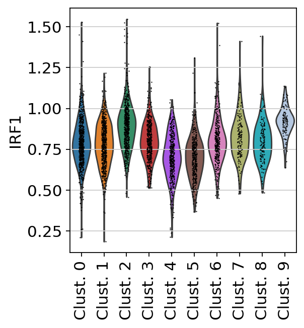
Here we observe the activity infered for IRF1 across spots. Interestingly, IRF1 is a known TF crucial for interferons-mediated signaling pathways. The inference of activities from “foot-prints” of target genes is more informative than just looking at the molecular readouts of a given TF, as an example here is the gene expression of IRF1, which is not very informative by itself:
[16]:
sc.pl.spatial(
    adata,
    color=['IRF1', 'leiden'],
    size=1.5,
    frameon=False
)
sc.pl.violin(
    adata,
    keys='IRF1',
    groupby='leiden',
    rotation=90
)
Exploration
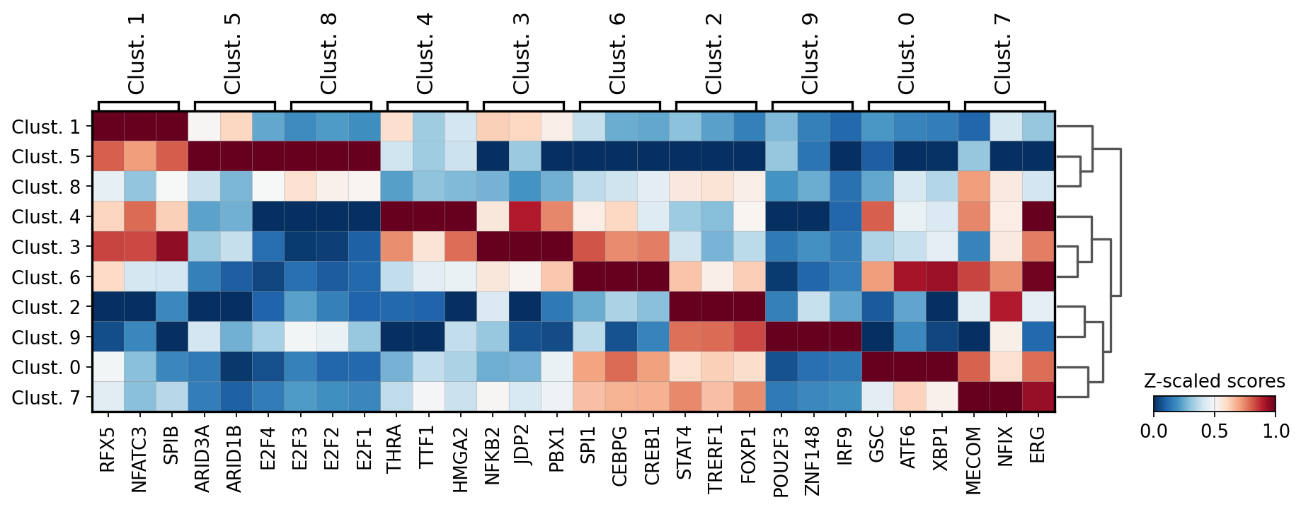
Let’s identify which are the top TF per cluster. We can do it by using the function dc.rank_sources_groups, which identifies marker TFs using the same statistical tests available in scanpy’s scanpy.tl.rank_genes_groups.
[17]:
df = dc.rank_sources_groups(acts, groupby='leiden', reference='rest', method='t-test_overestim_var')
df
[17]:
| group | reference | names | statistic | meanchange | pvals | pvals_adj | |
|---|---|---|---|---|---|---|---|
| 0 | Clust. 0 | rest | GSC | 26.693179 | 0.720106 | 3.805158e-127 | 1.358442e-124 |
| 1 | Clust. 0 | rest | ATF6 | 26.564711 | 0.806207 | 3.065348e-126 | 7.295529e-124 |
| 2 | Clust. 0 | rest | XBP1 | 26.303573 | 0.776220 | 2.330251e-124 | 4.159497e-122 |
| 3 | Clust. 0 | rest | TBXT | 24.935113 | 0.716476 | 5.946454e-114 | 8.491537e-112 |
| 4 | Clust. 0 | rest | PRDM1 | 23.248887 | 0.567659 | 8.897234e-101 | 1.058771e-98 |
| ... | ... | ... | ... | ... | ... | ... | ... |
| 7135 | Clust. 9 | rest | APEX1 | -12.681607 | -0.542233 | 7.593762e-28 | 2.464521e-26 |
| 7136 | Clust. 9 | rest | RFX1 | -12.708333 | -0.876288 | 3.256949e-28 | 1.162731e-26 |
| 7137 | Clust. 9 | rest | PREB | -12.731301 | -0.518973 | 3.112465e-28 | 1.162731e-26 |
| 7138 | Clust. 9 | rest | PITX1 | -14.683193 | -0.452296 | 1.235997e-34 | 5.515636e-33 |
| 7139 | Clust. 9 | rest | KAT2B | -20.452434 | -0.554208 | 7.525725e-51 | 7.676239e-49 |
7140 rows × 7 columns
We can then extract the top 3 markers per cluster:
[18]:
n_markers = 3
source_markers = df.groupby('group').head(n_markers).groupby('group')['names'].apply(lambda x: list(x)).to_dict()
source_markers
[18]:
{'Clust. 0': ['GSC', 'ATF6', 'XBP1'],
 'Clust. 1': ['RFX5', 'NFATC3', 'SPIB'],
 'Clust. 2': ['STAT4', 'TRERF1', 'FOXP1'],
 'Clust. 3': ['NFKB2', 'JDP2', 'PBX1'],
 'Clust. 4': ['THRA', 'TTF1', 'HMGA2'],
 'Clust. 5': ['ARID3A', 'ARID1B', 'E2F4'],
 'Clust. 6': ['SPI1', 'CEBPG', 'CREB1'],
 'Clust. 7': ['MECOM', 'NFIX', 'ERG'],
 'Clust. 8': ['E2F3', 'E2F2', 'E2F1'],
 'Clust. 9': ['POU2F3', 'ZNF148', 'IRF9']}
We can plot the obtained markers:
[19]:
sc.pl.matrixplot(acts, source_markers, 'leiden', dendrogram=True, standard_scale='var',
                 colorbar_title='Z-scaled scores', cmap='RdBu_r')
WARNING: dendrogram data not found (using key=dendrogram_leiden). Running `sc.tl.dendrogram` with default parameters. For fine tuning it is recommended to run `sc.tl.dendrogram` independently.
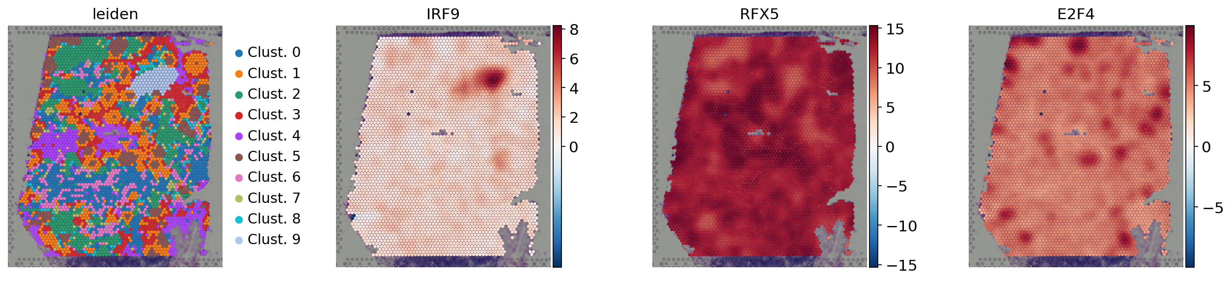
We can visualize again on the tissue some marker TFs:
[20]:
sc.pl.spatial(
    acts,
    color=['leiden', 'IRF9', 'RFX5', 'E2F4'],
    cmap='RdBu_r',
    size=1.5,
    vcenter=0,
    frameon=False
)
Pathway activity inference
We can also infer pathway activities from our transcriptomics data.
PROGENy model
PROGENy is a comprehensive resource containing a curated collection of pathways and their target genes, with weights for each interaction. For this example we will use the human weights (other organisms are available) and we will use the top 500 responsive genes ranked by p-value. Here is a brief description of each pathway:
Androgen: involved in the growth and development of the male reproductive organs.
EGFR: regulates growth, survival, migration, apoptosis, proliferation, and differentiation in mammalian cells
Estrogen: promotes the growth and development of the female reproductive organs.
Hypoxia: promotes angiogenesis and metabolic reprogramming when O2 levels are low.
JAK-STAT: involved in immunity, cell division, cell death, and tumor formation.
MAPK: integrates external signals and promotes cell growth and proliferation.
NFkB: regulates immune response, cytokine production and cell survival.
p53: regulates cell cycle, apoptosis, DNA repair and tumor suppression.
PI3K: promotes growth and proliferation.
TGFb: involved in development, homeostasis, and repair of most tissues.
TNFa: mediates haematopoiesis, immune surveillance, tumour regression and protection from infection.
Trail: induces apoptosis.
VEGF: mediates angiogenesis, vascular permeability, and cell migration.
WNT: regulates organ morphogenesis during development and tissue repair.
To access it we can use decoupler.
[21]:
progeny = dc.get_progeny(organism='human', top=500)
progeny
Downloading annotations for all proteins from the following resources: `['PROGENy']`
[21]:
| source | target | weight | p_value | |
|---|---|---|---|---|
| 0 | Androgen | TMPRSS2 | 11.490631 | 0.000000e+00 |
| 1 | Androgen | NKX3-1 | 10.622551 | 2.242078e-44 |
| 2 | Androgen | MBOAT2 | 10.472733 | 4.624285e-44 |
| 3 | Androgen | KLK2 | 10.176186 | 1.944414e-40 |
| 4 | Androgen | SARG | 11.386852 | 2.790209e-40 |
| ... | ... | ... | ... | ... |
| 6995 | p53 | ZMYM4 | -2.325752 | 1.522388e-06 |
| 6996 | p53 | CFDP1 | -1.628168 | 1.526045e-06 |
| 6997 | p53 | VPS37D | 2.309503 | 1.537098e-06 |
| 6998 | p53 | TEDC1 | -2.274823 | 1.547037e-06 |
| 6999 | p53 | CCDC138 | -3.205113 | 1.568160e-06 |
7000 rows × 4 columns
Activity inference with Multivariate Linear Model (MLM)
To infer pathway enrichment scores we will run the Multivariate Linear Model (mlm) method. For each spot in our slide (adata), it fits a linear model that predicts the observed gene expression based on all pathways’ Pathway-Gene interactions weights. Once fitted, the obtained t-values of the slopes are the scores. If it is positive, we interpret that the pathway is active and if it is negative we interpret that it is inactive.
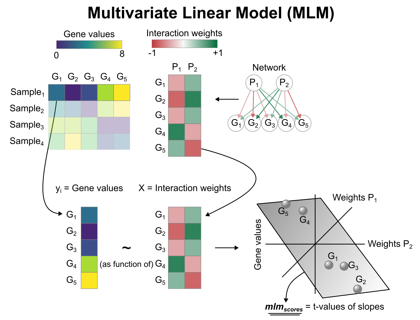
We can run mlm with a simple one-liner:
[22]:
dc.run_mlm(
    mat=adata,
    net=progeny,
    source='source',
    target='target',
    weight='weight',
    verbose=True,
    use_raw=False
)

# Store in new obsm keys
adata.obsm['progeny_mlm_estimate'] = adata.obsm['mlm_estimate'].copy()
adata.obsm['progeny_mlm_pvals'] = adata.obsm['mlm_pvals'].copy()
Running mlm on mat with 4032 samples and 19813 targets for 14 sources.
The obtained scores (t-values)(mlm_estimate) and p-values (mlm_pvals) are stored in the .obsm key:
[23]:
adata.obsm['progeny_mlm_estimate']
[23]:
| Androgen | EGFR | Estrogen | Hypoxia | JAK-STAT | MAPK | NFkB | PI3K | TGFb | TNFa | Trail | VEGF | WNT | p53 | |
|---|---|---|---|---|---|---|---|---|---|---|---|---|---|---|
| AAACAAGTATCTCCCA-1 | 0.726582 | 2.053643 | -1.000791 | 2.382140 | 6.987282 | -2.039776 | -0.701668 | -3.040569 | 0.064893 | 3.832963 | -2.758397 | 0.119536 | 0.258800 | -4.506958 |
| AAACAATCTACTAGCA-1 | 0.290291 | 1.083183 | -1.330531 | 2.192247 | 7.869350 | -2.282047 | -0.815247 | -3.588147 | -0.337527 | 3.434620 | -3.502797 | 0.230367 | 0.286089 | -4.556519 |
| AAACACCAATAACTGC-1 | 1.150137 | 2.426073 | -1.008912 | 2.499938 | 7.776049 | -2.682242 | -0.782385 | -3.192250 | 0.019723 | 3.800171 | -3.115057 | 0.243773 | 0.280674 | -4.311701 |
| AAACAGAGCGACTCCT-1 | 0.953800 | 2.201080 | -1.045912 | 1.849995 | 27.788458 | -2.363654 | -0.377379 | -2.606445 | -0.078141 | 3.240748 | -3.111001 | 0.055545 | 0.199865 | -5.400497 |
| AAACAGCTTTCAGAAG-1 | 0.525047 | 1.662629 | -1.394362 | 2.457380 | 6.697484 | -2.214217 | -1.591620 | -3.209660 | -0.590807 | 3.827924 | -2.293088 | -0.224760 | 0.807910 | -5.429735 |
| ... | ... | ... | ... | ... | ... | ... | ... | ... | ... | ... | ... | ... | ... | ... |
| TTGTTTCACATCCAGG-1 | 0.749198 | 2.242120 | -0.933600 | 2.753072 | 7.195352 | -2.574513 | -0.833506 | -3.092716 | -0.160780 | 3.545511 | -2.567993 | 0.151230 | 0.009297 | -4.479048 |
| TTGTTTCATTAGTCTA-1 | 0.789263 | 2.098119 | -1.414412 | 3.325075 | 7.465666 | -2.504934 | -0.525724 | -3.662633 | 0.119874 | 3.946503 | -2.805915 | 0.339055 | 0.133503 | -4.287980 |
| TTGTTTCCATACAACT-1 | 0.833514 | 1.983598 | -1.009022 | 2.609354 | 6.795700 | -2.645369 | -0.830475 | -2.940599 | 0.285104 | 3.994637 | -2.749641 | 0.056184 | 0.261842 | -4.687103 |
| TTGTTTGTATTACACG-1 | 0.792543 | 2.018600 | -1.130889 | 3.109919 | 8.298865 | -2.645617 | -0.529076 | -3.662524 | 0.480168 | 3.827680 | -2.748141 | -0.197740 | 0.338115 | -3.847667 |
| TTGTTTGTGTAAATTC-1 | 0.868652 | 1.681782 | -1.156972 | 2.128084 | 7.650702 | -2.521203 | -0.784943 | -3.557293 | -0.489564 | 3.589812 | -3.457454 | 0.164759 | 0.512957 | -4.315510 |
4032 rows × 14 columns
Visualization
Like in the previous section, we will extract the activities from the adata object.
[24]:
acts = dc.get_acts(adata, obsm_key='progeny_mlm_estimate')
acts
[24]:
AnnData object with n_obs × n_vars = 4032 × 14
    obs: 'in_tissue', 'array_row', 'array_col', 'n_genes', 'leiden', 'conn'
    uns: 'spatial', 'log1p', 'hvg', 'pca', 'neighbors', 'leiden', 'leiden_colors', 'dendrogram_leiden'
    obsm: 'spatial', 'X_pca', 'ulm_estimate', 'ulm_pvals', 'collectri_ulm_estimate', 'collectri_ulm_pvals', 'mlm_estimate', 'mlm_pvals', 'progeny_mlm_estimate', 'progeny_mlm_pvals'
Once extracted we can visualize them:
[25]:
sc.pl.spatial(
    acts,
    color=['Trail', 'leiden'],
    cmap='RdBu_r',
    vcenter=0,
    size=1.5,
    frameon=False
)
sc.pl.violin(
    acts,
    keys='Trail',
    groupby='leiden',
    rotation=90
)
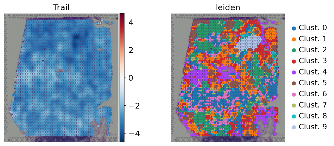
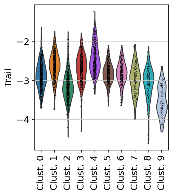
Here we show the activity of the pathway Trail, which is associated with apoptosis.
Exploration
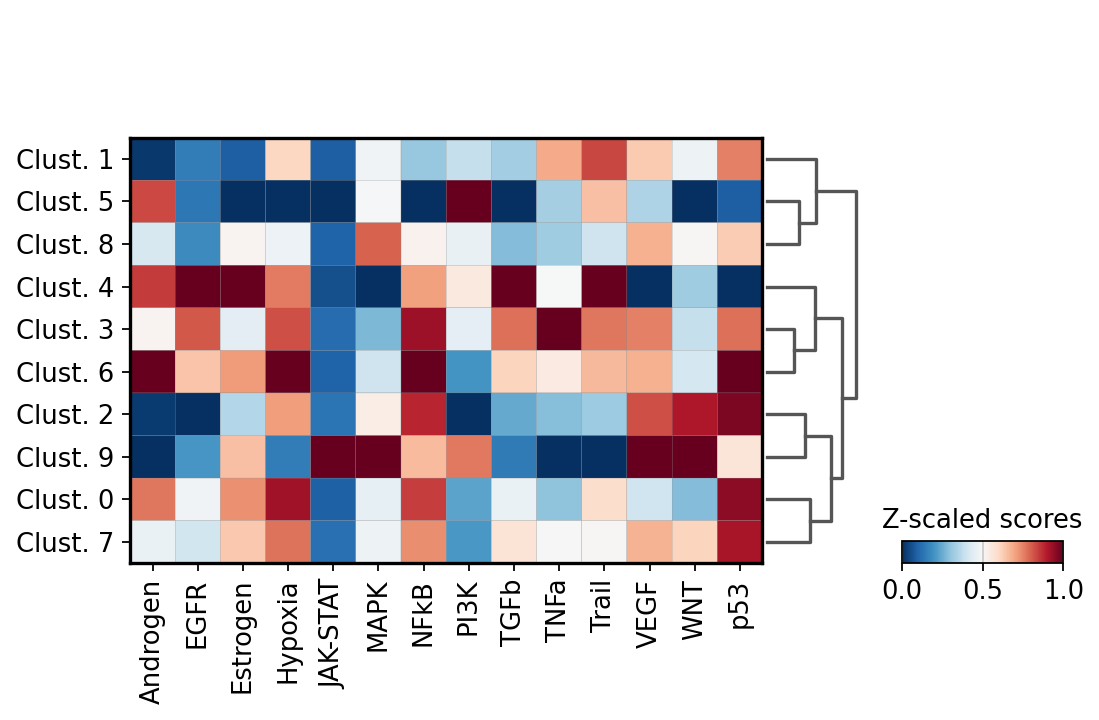
We can visualize which pathways are more active in each cluster:
[26]:
sc.pl.matrixplot(acts, var_names=acts.var_names, groupby='leiden', dendrogram=True, standard_scale='var',
                 colorbar_title='Z-scaled scores', cmap='RdBu_r')
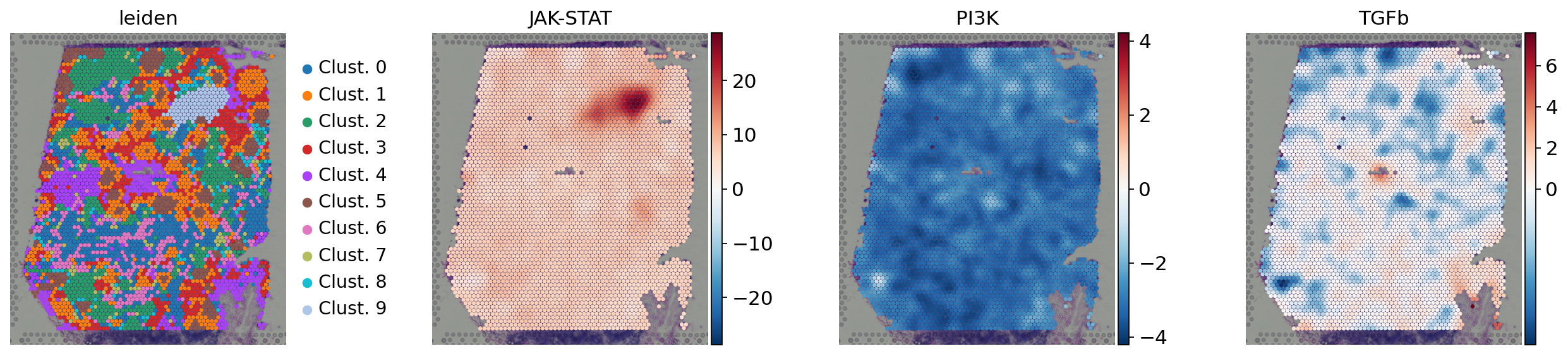
We can visualize again on the tissue some cluster-specific pathways:
[27]:
sc.pl.spatial(
    acts,
    color=['leiden', 'JAK-STAT', 'PI3K', 'TGFb'],
    cmap='RdBu_r',
    size=1.5,
    vcenter=0,
    frameon=False
)
Functional enrichment of biological terms
Finally, we can also infer activities for general biological terms or processes.
MSigDB gene sets
The Molecular Signatures Database (MSigDB) is a resource containing a collection of gene sets annotated to different biological processes.
[28]:
msigdb = dc.get_resource('MSigDB')
msigdb
Downloading annotations for all proteins from the following resources: `['MSigDB']`
[28]:
| genesymbol | collection | geneset | |
|---|---|---|---|
| 0 | MAFF | chemical_and_genetic_perturbations | BOYAULT_LIVER_CANCER_SUBCLASS_G56_DN |
| 1 | MAFF | chemical_and_genetic_perturbations | ELVIDGE_HYPOXIA_UP |
| 2 | MAFF | chemical_and_genetic_perturbations | NUYTTEN_NIPP1_TARGETS_DN |
| 3 | MAFF | immunesigdb | GSE17721_POLYIC_VS_GARDIQUIMOD_4H_BMDC_DN |
| 4 | MAFF | chemical_and_genetic_perturbations | SCHAEFFER_PROSTATE_DEVELOPMENT_12HR_UP |
| ... | ... | ... | ... |
| 3838543 | PRAMEF22 | go_biological_process | GOBP_POSITIVE_REGULATION_OF_CELL_POPULATION_PR... |
| 3838544 | PRAMEF22 | go_biological_process | GOBP_APOPTOTIC_PROCESS |
| 3838545 | PRAMEF22 | go_biological_process | GOBP_REGULATION_OF_CELL_DEATH |
| 3838546 | PRAMEF22 | go_biological_process | GOBP_NEGATIVE_REGULATION_OF_DEVELOPMENTAL_PROCESS |
| 3838547 | PRAMEF22 | go_biological_process | GOBP_NEGATIVE_REGULATION_OF_CELL_DEATH |
3838548 rows × 3 columns
As an example, we will use the hallmark gene sets, but we could have used any other.
Note
To see what other collections are available in MSigDB, type: msigdb['collection'].unique().
We can filter by for hallmark:
[29]:
# Filter by hallmark
msigdb = msigdb[msigdb['collection']=='hallmark']

# Remove duplicated entries
msigdb = msigdb[~msigdb.duplicated(['geneset', 'genesymbol'])]

# Rename
msigdb.loc[:, 'geneset'] = [name.split('HALLMARK_')[1] for name in msigdb['geneset']]

msigdb
[29]:
| genesymbol | collection | geneset | |
|---|---|---|---|
| 233 | MAFF | hallmark | IL2_STAT5_SIGNALING |
| 250 | MAFF | hallmark | COAGULATION |
| 270 | MAFF | hallmark | HYPOXIA |
| 373 | MAFF | hallmark | TNFA_SIGNALING_VIA_NFKB |
| 377 | MAFF | hallmark | COMPLEMENT |
| ... | ... | ... | ... |
| 1449668 | STXBP1 | hallmark | PANCREAS_BETA_CELLS |
| 1450315 | ELP4 | hallmark | PANCREAS_BETA_CELLS |
| 1450526 | GCG | hallmark | PANCREAS_BETA_CELLS |
| 1450731 | PCSK2 | hallmark | PANCREAS_BETA_CELLS |
| 1450916 | PAX6 | hallmark | PANCREAS_BETA_CELLS |
7318 rows × 3 columns
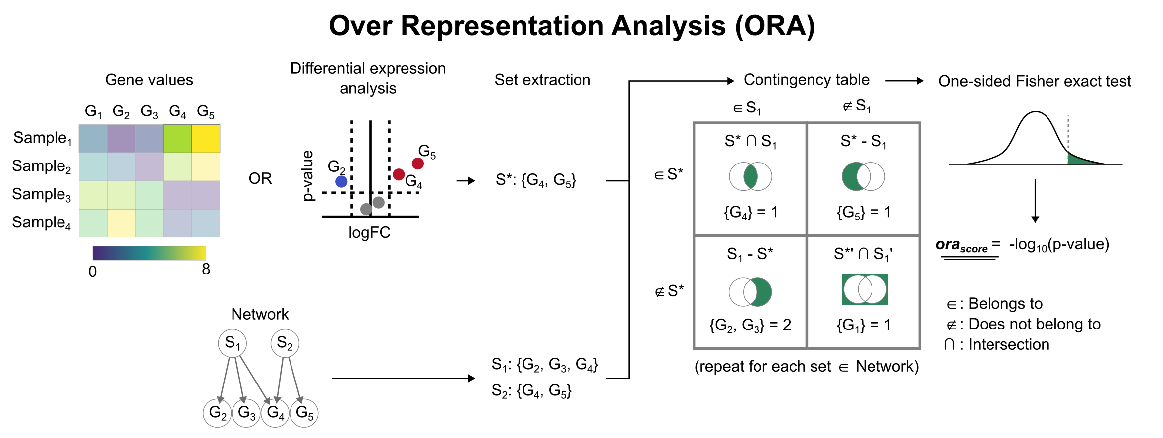
Enrichment with Over Representation Analysis (ORA)
To infer functional enrichment scores we will run the Over Representation Analysis (ora) method. As input data it accepts an expression matrix (decoupler.run_ora) or the results of differential expression analysis (decoupler.run_ora_df). For the former, by default the top 5% of expressed genes by sample are selected as the set of interest (S), and for the latter a user-defined significance filtering can be used. Once we have S, it builds a contingency table using set operations
for each set stored in the gene set resource being used (net). Using the contingency table, ora performs a one-sided Fisher exact test to test for significance of overlap between sets. The final score is obtained by log-transforming the obtained p-values, meaning that higher values are more significant.
We can run ora with a simple one-liner:
[30]:
dc.run_ora(
    mat=adata,
    net=msigdb,
    source='geneset',
    target='genesymbol',
    verbose=True,
    use_raw=False
)

# Store in a different key
adata.obsm['msigdb_ora_estimate'] = adata.obsm['ora_estimate'].copy()
adata.obsm['msigdb_ora_pvals'] = adata.obsm['ora_pvals'].copy()
Running ora on mat with 4032 samples and 19813 targets for 50 sources.
100%|████████████████████████████████████████████████████████████████████████████████████████████████████████████████████| 4032/4032 [00:08<00:00, 474.32it/s]
The obtained scores (-log10(p-value))(ora_estimate) and p-values (ora_pvals) are stored in the .obsm key:
[31]:
adata.obsm['msigdb_ora_estimate'].iloc[:, 0:5]
[31]:
| source | ADIPOGENESIS | ALLOGRAFT_REJECTION | ANDROGEN_RESPONSE | ANGIOGENESIS | APICAL_JUNCTION |
|---|---|---|---|---|---|
| AAACAAGTATCTCCCA-1 | 2.853878 | 27.778801 | 3.050313 | 0.626249 | 4.373918 |
| AAACAATCTACTAGCA-1 | 1.824514 | 28.717391 | 1.688825 | 0.626249 | 3.082310 |
| AAACACCAATAACTGC-1 | 3.242752 | 25.935842 | 2.558473 | 0.626249 | 3.491148 |
| AAACAGAGCGACTCCT-1 | 1.824514 | 31.600349 | 3.050313 | 0.294479 | 1.994681 |
| AAACAGCTTTCAGAAG-1 | 3.242752 | 21.533596 | 2.558473 | 0.294479 | 3.082310 |
| ... | ... | ... | ... | ... | ... |
| TTGTTTCACATCCAGG-1 | 2.853878 | 21.533596 | 3.050313 | 0.626249 | 1.994681 |
| TTGTTTCATTAGTCTA-1 | 3.653318 | 26.851581 | 4.138750 | 0.294479 | 3.082310 |
| TTGTTTCCATACAACT-1 | 4.084916 | 29.667245 | 2.558473 | 0.626249 | 2.696111 |
| TTGTTTGTATTACACG-1 | 2.144016 | 29.667245 | 2.103961 | 0.626249 | 3.082310 |
| TTGTTTGTGTAAATTC-1 | 1.824514 | 26.851581 | 3.577630 | 0.626249 | 3.082310 |
4032 rows × 5 columns
Visualization
Like in the previous sections, we will extract the activities from the adata object.
[32]:
acts = dc.get_acts(adata, obsm_key='msigdb_ora_estimate')

# We need to remove inf and set them to the maximum value observed
acts_v = acts.X.ravel()
max_e = np.nanmax(acts_v[np.isfinite(acts_v)])
acts.X[~np.isfinite(acts.X)] = max_e

acts
[32]:
AnnData object with n_obs × n_vars = 4032 × 50
    obs: 'in_tissue', 'array_row', 'array_col', 'n_genes', 'leiden', 'conn'
    uns: 'spatial', 'log1p', 'hvg', 'pca', 'neighbors', 'leiden', 'leiden_colors', 'dendrogram_leiden'
    obsm: 'spatial', 'X_pca', 'ulm_estimate', 'ulm_pvals', 'collectri_ulm_estimate', 'collectri_ulm_pvals', 'mlm_estimate', 'mlm_pvals', 'progeny_mlm_estimate', 'progeny_mlm_pvals', 'ora_estimate', 'ora_pvals', 'msigdb_ora_estimate', 'msigdb_ora_pvals'
Once extracted we can visualize them:
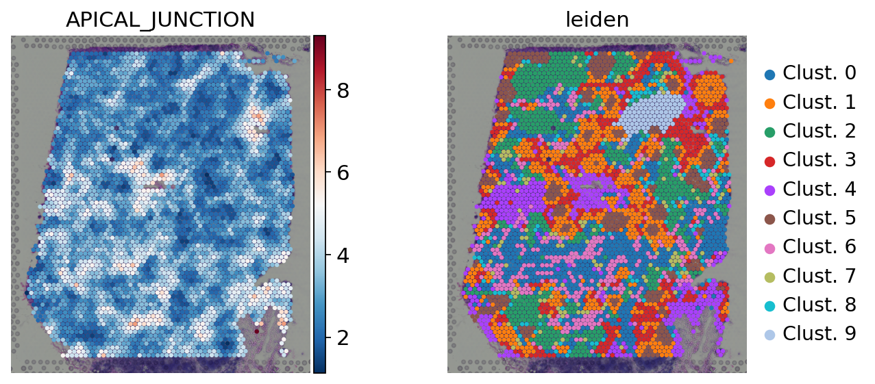
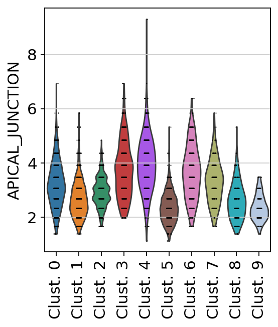
[33]:
sc.pl.spatial(
    acts,
    color=['APICAL_JUNCTION', 'leiden'],
    cmap='RdBu_r',
    size=1.5,
    frameon=False
)
sc.pl.violin(
    acts,
    keys='APICAL_JUNCTION',
    groupby='leiden',
    rotation=90
)
Exploration
Let’s identify which are the top terms per cluster. We can do it by using the function dc.rank_sources_groups, as shown before.
[34]:
df = dc.rank_sources_groups(acts, groupby='leiden', reference='rest', method='t-test_overestim_var')
df
[34]:
| group | reference | names | statistic | meanchange | pvals | pvals_adj | |
|---|---|---|---|---|---|---|---|
| 0 | Clust. 0 | rest | UNFOLDED_PROTEIN_RESPONSE | 11.159865 | 0.698623 | 9.250865e-28 | 4.625432e-26 |
| 1 | Clust. 0 | rest | UV_RESPONSE_UP | 9.698502 | 0.475151 | 1.473016e-21 | 1.841270e-20 |
| 2 | Clust. 0 | rest | HYPOXIA | 8.087560 | 0.635435 | 1.403690e-15 | 1.169741e-14 |
| 3 | Clust. 0 | rest | MTORC1_SIGNALING | 7.894915 | 0.677990 | 5.825152e-15 | 4.160823e-14 |
| 4 | Clust. 0 | rest | ANDROGEN_RESPONSE | 7.856351 | 0.295970 | 7.809971e-15 | 4.881232e-14 |
| ... | ... | ... | ... | ... | ... | ... | ... |
| 495 | Clust. 9 | rest | EPITHELIAL_MESENCHYMAL_TRANSITION | -7.434615 | -1.922915 | 6.866049e-12 | 3.120931e-11 |
| 496 | Clust. 9 | rest | APICAL_JUNCTION | -8.167614 | -0.809646 | 8.057563e-14 | 4.284914e-13 |
| 497 | Clust. 9 | rest | ESTROGEN_RESPONSE_LATE | -8.230622 | -0.314651 | 5.937254e-14 | 3.710784e-13 |
| 498 | Clust. 9 | rest | MITOTIC_SPINDLE | -8.510308 | -0.636282 | 5.161806e-15 | 3.687005e-14 |
| 499 | Clust. 9 | rest | TGF_BETA_SIGNALING | -10.227684 | -1.119047 | 4.436417e-20 | 5.545522e-19 |
500 rows × 7 columns
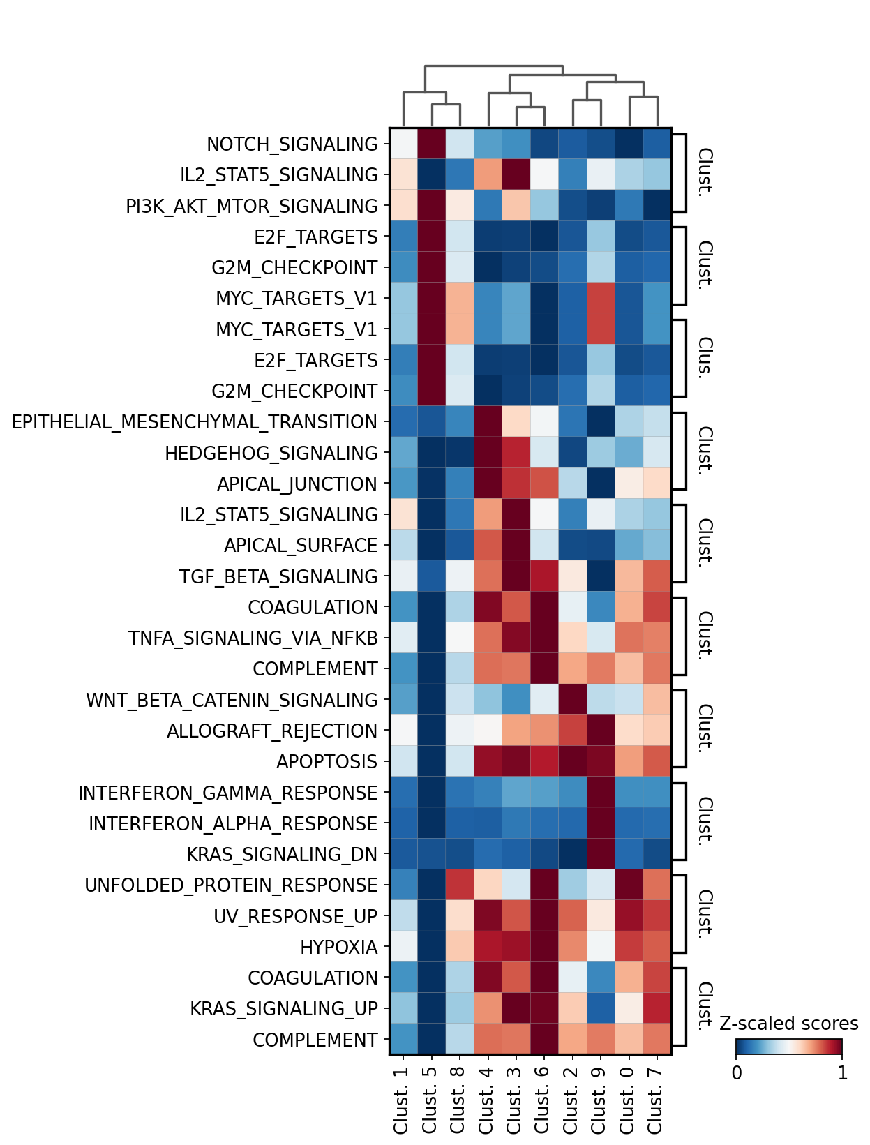
We can then extract the top 3 terms per cluster:
[35]:
n_top = 3
term_markers = df.groupby('group').head(n_top).groupby('group')['names'].apply(lambda x: list(x)).to_dict()
term_markers
[35]:
{'Clust. 0': ['UNFOLDED_PROTEIN_RESPONSE', 'UV_RESPONSE_UP', 'HYPOXIA'],
 'Clust. 1': ['NOTCH_SIGNALING',
  'IL2_STAT5_SIGNALING',
  'PI3K_AKT_MTOR_SIGNALING'],
 'Clust. 2': ['WNT_BETA_CATENIN_SIGNALING',
  'ALLOGRAFT_REJECTION',
  'APOPTOSIS'],
 'Clust. 3': ['IL2_STAT5_SIGNALING', 'APICAL_SURFACE', 'TGF_BETA_SIGNALING'],
 'Clust. 4': ['EPITHELIAL_MESENCHYMAL_TRANSITION',
  'HEDGEHOG_SIGNALING',
  'APICAL_JUNCTION'],
 'Clust. 5': ['E2F_TARGETS', 'G2M_CHECKPOINT', 'MYC_TARGETS_V1'],
 'Clust. 6': ['COAGULATION', 'TNFA_SIGNALING_VIA_NFKB', 'COMPLEMENT'],
 'Clust. 7': ['COAGULATION', 'KRAS_SIGNALING_UP', 'COMPLEMENT'],
 'Clust. 8': ['MYC_TARGETS_V1', 'E2F_TARGETS', 'G2M_CHECKPOINT'],
 'Clust. 9': ['INTERFERON_GAMMA_RESPONSE',
  'INTERFERON_ALPHA_RESPONSE',
  'KRAS_SIGNALING_DN']}
We can plot the obtained terms:
[36]:
sc.pl.matrixplot(acts, term_markers, 'leiden', dendrogram=True, standard_scale='var',
                 colorbar_title='Z-scaled scores', cmap='RdBu_r', swap_axes=True)
We can visualize again on the tissue some cluster-specific terms:
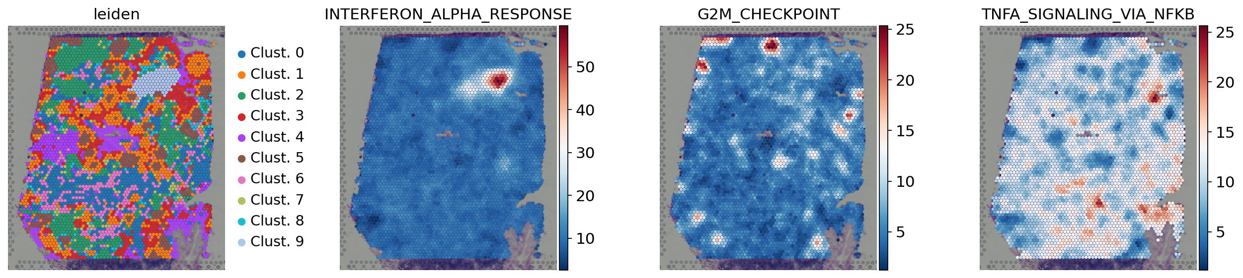
[37]:
sc.pl.spatial(
    acts,
    color=['leiden', 'INTERFERON_ALPHA_RESPONSE', 'G2M_CHECKPOINT','TNFA_SIGNALING_VIA_NFKB'],
    cmap='RdBu_r',
    size=1.5,
    frameon=False
)